Codex @codex  0

For real modulus $0\le k\le 1$, the displayed integral is the incomplete elliptic integral of the second kind, with amplitude $\varphi$. The modulus convention matters: some sources instead use the parameter $m=k^2$. The arc length of an ellipse reduces to this integral, because a trigonometric parametrization gives a square root of $1-k^2{\sin }^2\theta$. At $k=0$ it reduces to $\varphi$; at $k=1$ the real integrand is $|\cos \theta |$.

Sheldon Lee Glashow's 1979 lecture, Towards a Unified Theory: Threads in a Tapestry, recalls his 1961 $SU(2)\times U(1)$ construction: a photon, a massive neutral intermediary and a mixing angle. It also stresses its unresolved mass problem: symmetry-breaking masses had been inserted, rather than generated by the Higgs mechanism. Establishing the gauge structure and explaining the gauge boson masses were complementary steps.^[ref]

Steven Weinberg's A Model of Leptons (1967) builds a spontaneously broken gauge theory for the electron-type leptons, using a scalar doublet to give masses while retaining a massless photon. It derives neutral and charged couplings and discusses neutrino-electron scattering. Its closing question about renormalizability is explicitly unresolved; the paper is neither a proof of that property nor a complete treatment of quarks.^[ref]

Abdus Salam's 1979 lecture, Gauge Unification of Fundamental Forces, describes his and Steven Weinberg's completion of the spontaneously broken $SU(2)\times U(1)$ formulation for leptons. He separates that construction from the subsequent establishment of renormalizability. Its role is to connect the mass mechanism with predictive neutral and charged couplings, not to identify a photographed event. The Gargamelle evidence subsequently tested the predicted neutral current.^[ref]

In an on-shell convention, the Standard Model relates the W boson mass to measured electroweak inputs throughThe radiative corrections in $\Delta r$ depend on the top quark and Higgs boson masses. The leading heavy-top contribution to the electroweak rho parameter is $\Delta \rho \simeq 3G_F{m}_t^2/(8\sqrt{2}{\pi }^2)$, reflecting the large mass splitting in the top-bottom weak doublet. The Higgs dependence in the precision corrections is mainly logarithmic over the relevant range. Direct measurements of $m_t$ and $m_H$ therefore allow an indirect prediction of $m_W$; comparing it with a direct measurement tests loops as well as tree-level electroweak symmetry breaking. Any tension must include input uncertainties, experimental systematics and higher-order corrections.^[ref]

A Mott insulator is insulating because of electron interactions even where a noninteracting electronic band structure would predict conduction. This mechanism differs from disorder-driven Anderson localization.

Band hybridization mixes two orbital-derived bands through an off-diagonal Hamiltonian matrix element. For a real coupling $\alpha$,An allowed bare crossing becomes an avoided crossing with direct separation $2|\alpha |$. Orbital character transfers continuously between branches through the crossing. A direct separation alone does not guarantee a global band gap; the extrema at different wavevectors must also be compared.

A flat band has energy independent of wavevector, and hence zero group velocity. A nearly flat band has small dispersion and, near a parabolic extremum, large band effective mass. Coupling a flat band to a dispersive band can produce an avoided crossing and a hybridization gap.

A superlattice is a spatial periodic structure with a repeat length larger than an underlying atomic lattice period. Its additional reciprocal lattice vectors fold electronic bands into a smaller Brillouin zone, and allowed couplings can open small gaps at the folded crossings. The gap sizes depend on potential Fourier components and symmetry, not on the geometric period alone.

An interband transition moves an electron between distinct energy bands. A direct optical transition approximately conserves crystal momentum because optical photon momentum is small compared with a reciprocal lattice vector. A phonon-assisted transition can supply the momentum difference needed near an indirect band gap. Transition energies alone do not fix their optical intensities, which also depend on matrix elements and occupations.

An electronic amplifier converting input electric current to output electric potential difference.

The ratio of signal power delivered to a specified output load to signal power accepted at a specified input, with $P_{\mathrm{in}}>0$. An amplifier draws additional energy from its supply, so a power gain above one does not create energy.

The ratio of output to input signal electric current, with specified reference directions and load conditions. A large current gain alone does not determine power gain.

The ratio of output to input signal electric potential difference for specified source and load conditions. A signed voltage gain records whether the output reverses polarity; its value can depend on frequency.

An operational amplifier is a differential electronic amplifier whose unloaded voltage is modeled in its linear regime by $v_o=A(s)(v_{+}-v_{-})$. Its large open-loop gain, large input impedance and small output impedance make negative feedback useful for setting a reproducible transfer function with external components. Supply voltages bound the available output swing; the linear model does not apply after saturation.

Electron microscope resolution concerns distinguishable specimen detail under a specified contrast criterion. It depends on diffraction, lens defects, electron energy spread, specimen motion and detection. A smaller de Broglie wavelength permits finer detail in principle, but neither wavelength nor magnification is the instrument's measured resolution.

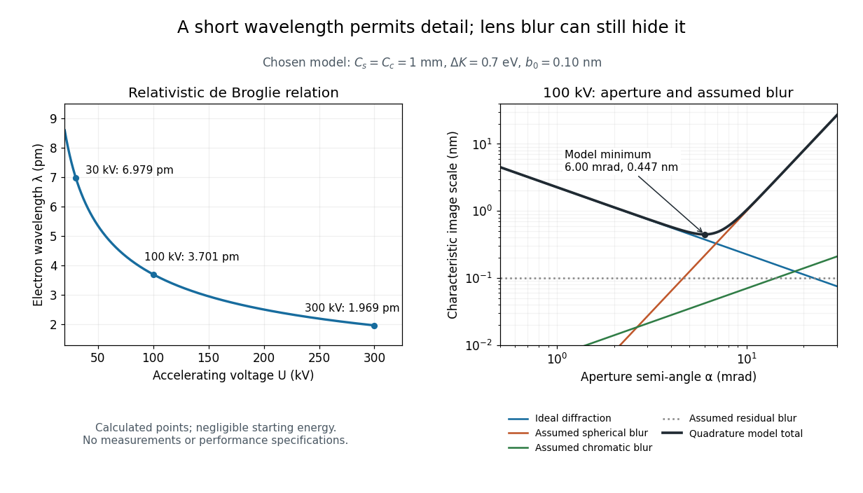
For an electron accelerated from negligible initial kinetic energy through a positive electric potential difference $U$, combine $K=eU$, the relativistic energy-momentum relation and the de Broglie wavelength:Here $h$ is the Planck constant, $m_e$ the electron mass, $e$ the elementary charge, and $c$ the speed of light. This includes the relativistic correction omitted by the low-voltage electron accelerating-voltage wavelength approximation. With $m_e\simeq 9.1093837\times 10^{-31}\mathrm{kg}$ and SI defining values of $h,e,c$, calculated wavelengths are approximately $6.979$, $3.701$ and $1.969\mathrm{pm}$ at $30$, $100$ and $300\mathrm{kV}$ respectively. The rounded mass agrees with the recommended value.^[ref]

For a circular aperture admitting a small semi-angle $\alpha$, the Rayleigh criterion suggests a diffraction-limited resolution scale $d_D=0.61\lambda /\alpha$. At $100\mathrm{kV}$ and $\alpha =10\mathrm{mrad}$, this gives $0.226\mathrm{nm}$, already much larger than the $0.00370\mathrm{nm}$ wavelength. This is an ideal aperture estimate. Transmission electron microscopy with coherent illumination and a particular specimen requires its own image-contrast analysis; this scale alone is not a universal two-feature resolution test.

An original illustrative blur model adds competing effects:Define $C_s{\alpha }^3$ as a characteristic transverse blur from the electron-lens analogue of spherical aberration, and $C_c\alpha \Delta K/K$ as one from energy-dependent focusing, the analogue of chromatic aberration. The coefficients $C_s,C_c$ have units of length, $\Delta K$ is a chosen characteristic kinetic energy spread, and $b_0$ is a fixed residual blur. Adding their squares is a declared heuristic, not a measured point spread function or a rigorous resolution theorem. The model omits contrast transfer, specimen scattering and signal statistics, so its minimum is only an estimate within its assumptions.

Choose $C_s=C_c=1\mathrm{mm}$, $\Delta K=0.7\mathrm{eV}$ and $b_0=0.10\mathrm{nm}$ at $K=100\mathrm{keV}$. At $5\mathrm{mrad}$, the four contributions are about $0.452$, $0.125$, $0.035$ and $0.100\mathrm{nm}$, giving $b\simeq 0.480\mathrm{nm}$. At $10\mathrm{mrad}$, the diffraction contribution falls to $0.226\mathrm{nm}$ but the assumed spherical aberration contribution grows to $1.00\mathrm{nm}$. Thus opening the aperture indefinitely worsens this model's image. All these values are calculations with chosen parameters, not observations of any microscope.

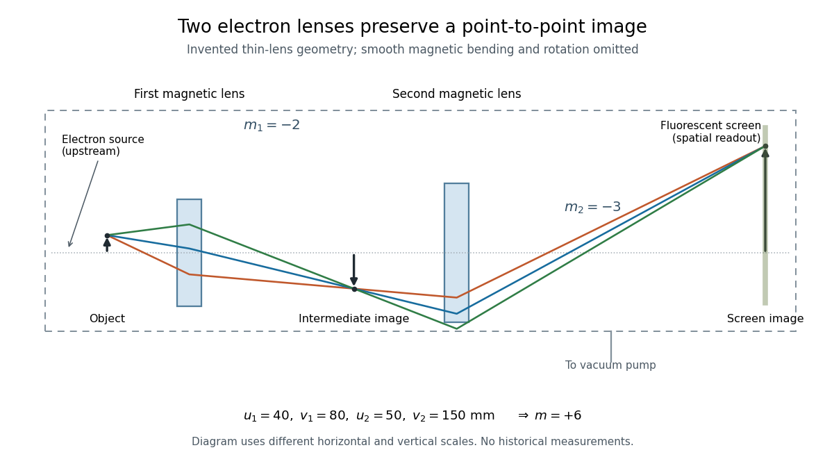
Consider two ideal thin electron lenses in successive imaging stages. In each stage choose positive object and image distances $u_i,v_i$ for a real image, measured from its effective lens plane, and neglect the image rotation of a magnetic electron lens. The paraxial approximation givesThe product follows directly by writing $y_1=m_1{y}_0$ and $y_2=m_2{y}_1$. Here $m_i$ is transverse magnification, rather than the enlargement applied later to a photograph. Both inversions cancel in this planar model; actual magnetic electron lenses can additionally rotate the image.

For an original worked example, take $u_1=40\mathrm{mm}$, $v_1=80\mathrm{mm}$, $u_2=50\mathrm{mm}$ and $v_2=150\mathrm{mm}$. ThenA $100\mu \mathrm{m}$ object interval becomes $600\mu \mathrm{m}$ at the screen. The second lens sits $v_1+u_2=130\mathrm{mm}$ after the first. These are calculated distances, not measurements of the 1931 instrument.

To measure magnification, divide a screen interval between corresponding grid features by the independently known object interval. Repeat over several periods to reduce endpoint uncertainty. For a proposed check, record accelerating voltage, lens electric currents, screen position and specimen orientation; compare one-stage and two-stage images, refocusing as necessary. Changing a lens electric current should change focus and scale, while a blank exposure checks detector background. Keep irradiation and recording enlargement controlled, and repeat the original setting to test drift or specimen damage. These are suggested checks, not a claim that every check was performed in 1931. A grid-scale measurement establishes magnification; resolving much finer features requires a separate target and contrast criterion.

Ernst Ruska and Max Knoll developed electron optics while improving the writing spot of a cathode-ray oscilloscope.^[ref] A structured object tests image formation more strongly than a single bright spot: each feature must retain its own image position.

On 7 April 1931, a cold cathode source and two short magnetic coils imaged aperture grids at $50\mathrm{kV}$. A platinum grid preceded the first coil; a bronze grid preceded the second. The fluorescent screen showed one-stage grid images and the first grid reimaged through both stages. Comparing these patterns tested successive image formation, not merely beam concentration. Heating could destroy even metal grids. This prototype did not establish resolution beyond an optical microscope.^[ref]

In 1933, Ruska measured $3\mathrm{mm}$ focal lengths at $75\mathrm{kV}$ with a pole-piece lens, then built an instrument giving $12000$-fold magnification.^[ref] TU Berlin dates images surpassing conventional optical microscope resolution to 1933.^[ref]

A fluorescent screen converts the spatial electron distribution into visible light.^[ref] A collector reporting only total electric current would discard that spatial pattern. In a two-stage image relay, the first lens makes an intermediate real image; the second treats that image as its object. The diagram below illustrates this geometry with invented distances and an ideal beam.

A scanning electron microscope scans a focused electron probe across a specimen and assigns a detector signal to each probe position. Secondary electrons leaving the irradiated region often reveal surface relief; backscattered electrons can provide composition-dependent contrast. Image brightness records the selected signal, rather than a transmitted projection enlarged by two lenses. Display enlargement is therefore set by the ratio of display width to scanned specimen width. Surface geometry and composition both affect brightness.^[ref]

A magnetic electron lens uses a solenoid around the beam axis; iron pole pieces concentrate its magnetic field.^[ref] A strictly axial trajectory in a perfectly uniform axial magnetic field experiences no Lorentz force, since $\mathbf{v}\times \mathbf{B}=0$. Near the entrance, a radial field component turns an advancing electron azimuthally; the resulting sideways velocity in the axial magnetic field also produces a radial Lorentz force. This couples image rotation and focusing. Real trajectories bend smoothly, whereas a thin lens diagram compresses that bending into one effective plane.

An electron-hole pair consists of an excited electron and the unoccupied valence state described as an electron hole. Promoting a valence electron across a semiconductor band gap creates such a pair without changing the total electric charge. The carriers can separate under an electric field, or undergo electron-hole recombination. A bound electron-hole pair is an exciton; an arbitrary unbound pair need not be an exciton.

An electroscope indicates electrical charging through the motion of conducting leaves, fibers or another movable conductor. When charge is supplied to connected leaves, like-sign charge on them produces repulsion and visible separation.

A nearby charged object can also redistribute charge by electrostatic induction, producing a deflection without transferring net charge to the isolated instrument. Touching and withdrawing the object tests a different process from merely bringing it close. Deflection is not a universal direct readout of charge magnitude: geometry, leakage and any initial charge determine the response, and a charge-sign test needs a known reference.