
Equivalence of group representations Created 2026-10-18 Updated 2026-10-20
Two finite-dimensional group representations over the same field are equivalent if there is one invertible linear map intertwining all their group actions, equivalently for every . The same change of basis must work simultaneously for all group elements. The cyclic property of the trace implies that equivalent representations have identical characters: . Consequently a difference at a single group element proves inequivalence. This implication does not need the group to be finite, and the reverse implication is not asserted for arbitrary groups or fields.
Shifted addition on odd integers 2026-10-18
The odd integers form an abelian group under the displayed operation. The identity element is and the inverse element of is . The bijection is a group isomorphism to , since it converts the shifted operation into addition. This illustrates how an unfamiliar identity and inverse can arise from ordinary addition by a change of coordinates.
Exact factorization of a group Created 2026-10-18 Updated 2026-10-31
Two subgroups give an exact factorization of a group when every element has a unique expression with . Existence and trivial intersection are equivalent to this uniqueness: if , then , so both sides are the identity. Conversely, an element in the intersection gives the two factorizations , forcing . For finite groups the multiplication map is therefore a bijection and . It need not be a group homomorphism: an exact factorization is not automatically a direct product of groups. If is normal, it gives an internal semidirect product.
An inviscid uniform-density self-gravitating cylinder in vacuum, with no rotation or surface tension, has the displayed axisymmetric dispersion relation, where . To derive it, let . The linear kinematic boundary condition gives . The Lagrangian pressure perturbation vanishes on the moving free surface, giving . Substitute the axisymmetric gravitational potential of a displaced cylindrical interface and use to obtain the relation. Its nonzero neutral root is : wavelengths longer than have and grow. The fastest-growing mode has , so its wavelength is about . Negative must be interpreted through an imaginary frequency, not through a real oscillatory ansatz.
Gate control of graphene carrier density Created 2026-10-18 Updated 2026-10-20
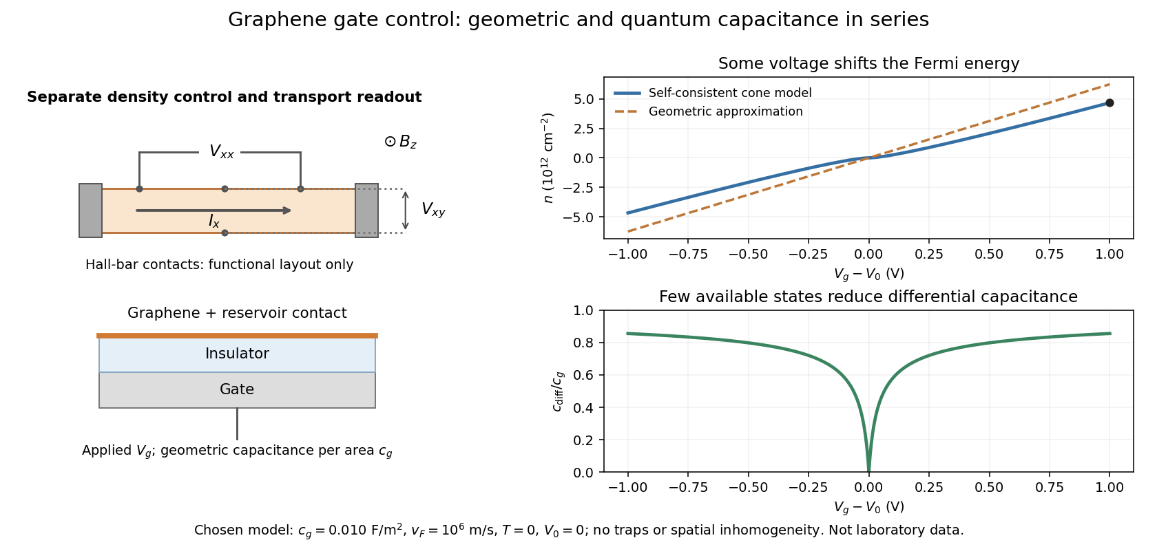
Consider an ideal uniform graphene sheet connected to an electron reservoir, with an insulated gate. Let be geometric capacitance per unit area, the elementary charge, and the neutral-point offset. Neglect temperature, trapped electric charge and spatial inhomogeneity. A change in gate voltage pays for both the electrostatic potential drop, , and the change in the sheet's Fermi energy, . Here is measured relative to the band crossing; it is negative for excess electron holes.
Combine this relation with the carrier density in a graphene cone. Write , measured in volts, , and . ThenThe positive root is unique because is strictly increasing for . The often useful geometric approximation neglects the Fermi energy term. It overestimates in this model, especially near neutrality where relatively few states are available.
For a deliberately chosen model with , , and , the formulas give and . The purely geometric value would be . These are chosen-model predictions, not measurements of the historical devices. Numerical conversion uses the exact Planck constant and elementary charge.[ref]
Fundamental Physical Constants — Complete Listing by National Institute of Standards and Technology and others. Exact h and e entries; material parameters in this example are stipulated
Andre Geim, Konstantin Novoselov and collaborators mechanically cleaved graphite, identified thin flakes, and fabricated multi-terminal Hall bars on oxidized silicon. A substrate gate changed the carrier density; longitudinal electrical resistance and the Hall coefficient supplied different checks. The 2004 report included one-, two- and three-layer devices and described a few-layer semimetal interpretation. Layer identification and electrical control were separate experimental achievements.[ref]
Electric Field Effect in Atomically Thin Carbon Films by Konstantin Novoselov and others. pp.1–2 and Figs.1–2: preparation, thickness selection and electrical measurements
The 2005 monolayer study used an optical microscope, electron microscopy and atomic force microscopy to select monolayers. It then measured Shubnikov-de Haas oscillations as temperature, gate voltage and magnetic field varied. Their damping inferred a density-dependent cyclotron effective mass; comparison with oscillation frequency tested a linear dispersion relation. A comparison with two-layer devices also distinguished their quantum Hall effect sequences. These are complementary tests of the monolayer model, rather than consequences of finding a thin-looking flake alone.[ref]
Two-Dimensional Gas of Massless Dirac Fermions in Graphene by Konstantin Novoselov and others. pp.1–3, Figs.2–4: monolayer selection, oscillation damping and bilayer comparison
Nearest-neighbour model of graphene Created 2026-10-18 Updated 2026-10-20
Take a planar honeycomb lattice with two sites per primitive cell and one localized atomic orbital per site. In this explicitly idealized tight-binding model, all three nearest-neighbour hopping matrix elements are , with ; there is no on-site offset or further-neighbour hopping. Ignore electron interactions and treat physical spin as a separate degeneracy. Let the bond length be , and choose the three vectors from an site to its neighbours asThe Bloch state amplitudes on form a two-component vector. A consistent phase convention gives the HamiltonianIts characteristic equation is , giving the two displayed energy bands. The two-component structure comes from the two sites, rather than two values of physical spin. This is a particularly small matrix model in which a crystal's geometry creates an unexpected low-energy law.
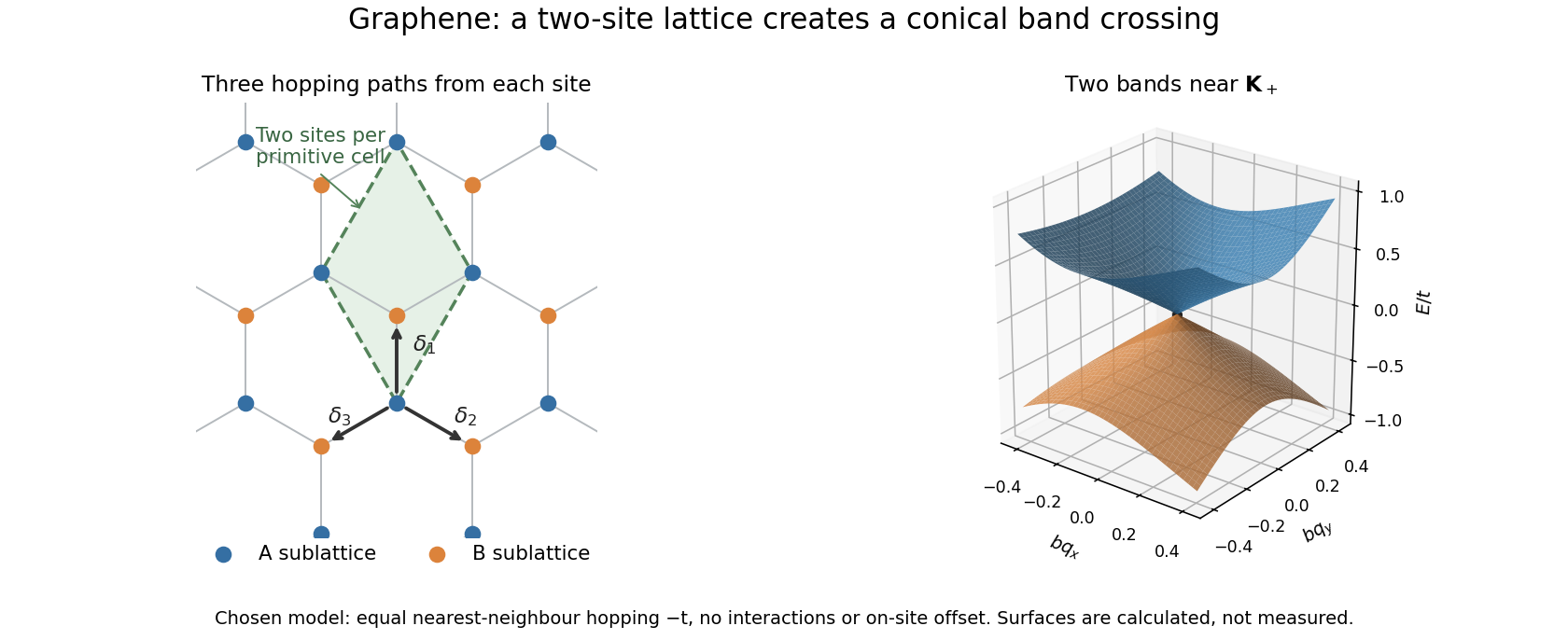
A honeycomb lattice produces two touching electronic bands
. Original nearest-neighbour model with the defined bond vectors. The surface shows the calculated bands near one zero of , with distance in units of inverse bond length and energy in units of the hopping magnitude. These are model energies, not measured band data. Source. Details.Historically, Philip Russell Wallace used a tight-binding model to investigate the electronic band structure of graphite in 1947. The material in that paper was layered graphite; the single-sheet model here isolates one simpler part of the problem.[ref]
The Band Theory of Graphite by Philip Russell Wallace. Publisher abstract: tight-binding bands and Brillouin zones of graphite; published 1 May 1947
Fixed-step gradient descent on a positive-definite quadratic Created 2026-10-18 Updated 2026-10-25
Consider the original two-dimensional exampleThe Hessian matrix is , a symmetric matrix and positive-definite matrix. Its eigenvectors are the coordinate directions, its eigenvalues are and , and its Euclidean norm condition number is . The unique global minimum is , so the error equals . The linear map , with the identity matrix, givesFor , the two coordinate error multipliers are and . Consequently , , and the second coordinate changes sign at every step while both shrink. The Euclidean norm of the error contracts by each step. The objective gap, which we call the quadratic energy, contracts by its square:The level sets of are ellipses. Oscillation across their narrow direction is compatible with strictly decreasing energy.
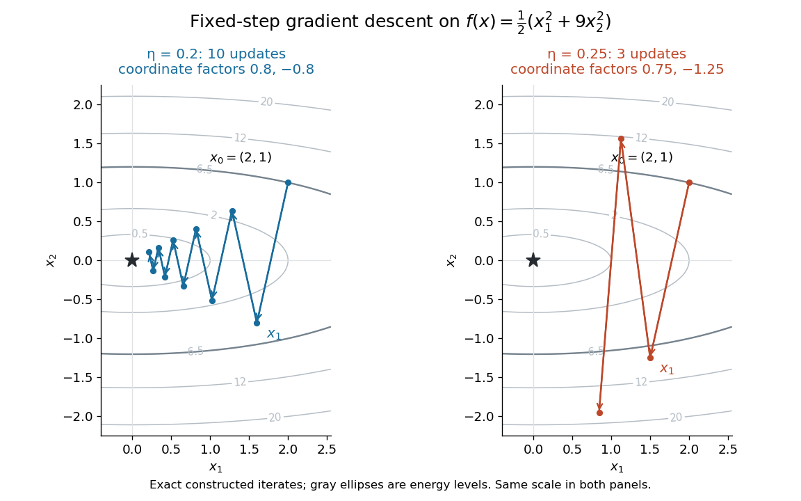
Original gradient descent iterates on : step size contracts both directions, whereas expands the second
. Details. For , the coordinate error multipliers become and , giving . The first coordinate still tends to zero, but the second alternates and grows. Direct substitution givesThus a larger positive step size can turn a strictly convex function into a divergent iteration. Energy and error are different quantities: coordinate errors carry signed multipliers, while each coordinate's contribution to energy carries the squared multiplier.
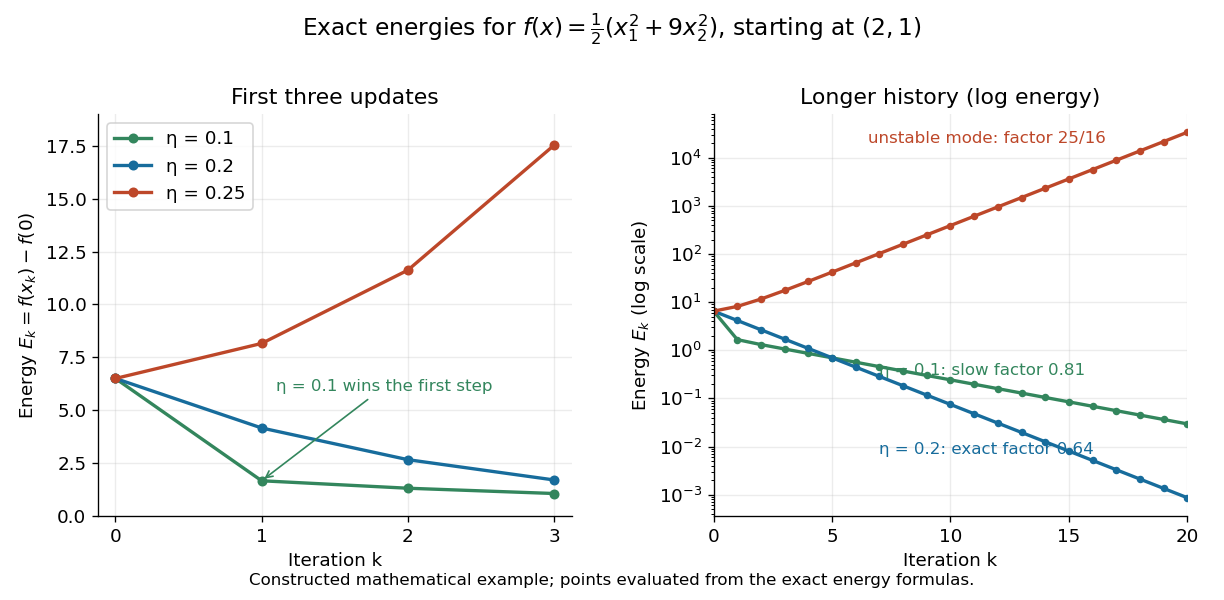


For the general quadratic form with linear termthe error obeys the same linear map . The spectral theorem for real symmetric matrices supplies an orthonormal basis of eigenvectors with positive eigenvalues . Writing gives the exact solution and energy identityTherefore convergence from every initial vector is equivalent toAt , a nonzero error component along a largest-eigenvalue eigenvector flips sign without shrinking. Above that threshold it grows. A particular start can still converge if it has zero components in every unstable direction; the interval is the condition for all starts. If , then and . These bounds follow by summing the squared components in the orthonormal basis.
Golgi lumen 2026-10-18
The Golgi lumen is the enclosed interior of a Golgi cisterna, distinct from the surrounding cytosol.
The membrane-sidedness rule in secretory protein routing still applies within the Golgi apparatus. For a local worked example, stipulate a membrane protein with a carbohydrate chain exposed to Golgi lumen and a tail exposed to cytosol. An enzyme confined to Golgi lumen can contact that chain, but cannot directly contact the cytosolic tail without a boundary-crossing step. A change in which Golgi cisterna contains the protein need not turn the protein over. Thus chemical accessibility and cargo location are different questions: moving cargo onward preserves its membrane sides under the budding and fusion operations described in secretory protein routing.
Upper critical magnetic field 2026-10-18
Linearize the stated model about in a uniform magnetic field. The kinetic operator has the Landau level ground energy . Its cancellation with givesThis is the bulk orbital field scale of this model; it excludes spin-polarization limits and uses the normal-state relation . For the chosen , it is about . With , . Counting triangular cells at would give , but it is the linearized field equation, rather than disks of an arbitrarily chosen core radius touching, that supplied the transition criterion.
Lower critical magnetic field 2026-10-18
The applied bulk magnetic field at which introducing a vortex first becomes favorable in the ideal equilibrium type-II problem. Surface barriers, sample shape and flux pinning can change the apparent entry field.
Ginzburg-Landau parameter 2026-10-18
In the isotropic single-component model, gives the type-I regime and the type-II regime; the interface-energy distinction belongs to the model, rather than a purely geometric test of core overlap.[ref]
Nobel Lecture: Type-II superconductors and the vortex lattice by Alexei Alexeyevich Abrikosov. p.975, interface energy and the type-II regime
Superconducting coherence length Created 2026-10-18 Updated 2026-10-20
The gradient and quadratic terms of the stated model balance at the amplitude-variation scale . It is a superconducting length scale, distinct from optical coherence length. The weak-field London penetration depth in the same normalization obeysA core suppresses the pairing amplitude over a scale set by ; screening electric currents and the magnetic field involve . Neither scale is a universal particle size.
A concrete motivating experiment is the acetone–chloroform mixture in Truman State University's Liquid-Vapor Equilibrium of a Binary System, Procedure and Figure 1. A two-neck flask feeds a distillation head with a water-cooled laboratory condenser, condensate sampling arm and temperature probe. Starting with one pure liquid, the procedure adds the other component successively and waits for stable temperature with returning condensate. Small paired samples from the flask and condensate are read on an Abbé refractometer; a tabulated refractive index–composition relation gives the two compositions. Controls include three-point thermometer calibration, corrected atmospheric pressure readings, and agreement of the initial pure-liquid and condensate refractive indices with the reference value. Small withdrawals and little retained condensate reduce disturbance of composition. Sample evaporation can bias the readout. The inferred paired mole fractions, temperature and pressure describe vapor-liquid equilibrium, subject to the conversion from mass fraction to mole fraction and to representative sampling. This teaching protocol reports no measured results of a particular student run.[ref]
How does such a measurement expose activity coefficients? Let and be the mole fractions in the liquid and gas thermodynamic phases, respectively, and let be the pure-component vapor pressure. Assume the gas thermodynamic phase is an ideal gas mixture and neglect the change of the pure-liquid reference chemical potential between its saturation pressure and the experimental pressure. Equality of each component's chemical potential between the two thermodynamic phases then givesThis turns the paired composition readings into estimates of the activity coefficients. The approximation needs refinement when the gas departs appreciably from ideal gas behavior or the neglected liquid pressure effect matters.
The apparatus measures a boiling-composition series in which temperature changes as the mixture changes. Its readings therefore cannot be inserted directly into the fixed-temperature, fixed-pressure activity coefficient constraint. They motivate the more general task: test whether the measured mixture properties can arise from a common Gibbs free energy while accounting for changing state variables. A failure can reveal incompatible property fits or experimental bias; a pass supplies a consistency check, not proof that every reading is correct.
Binary activity-coefficient consistency 2026-10-18
For a nonideal chemical solution, write its thermodynamic activities on a mole fraction basis as and . Use composition-independent pure-component reference chemical potentials at the same temperature and pressure:The activity coefficients describe departure from the ideal solution under that reference convention.[ref]
At fixed temperature and pressure, insert these expressions into the Gibbs-Duhem equation. The ideal solution terms cancel because . What remains isThus two independent fits to measured activity coefficients can each look smooth while failing to describe one possible Gibbs free energy. This is a necessary consistency condition; satisfying it alone does not establish experimental accuracy or thermodynamic stability.
For an original algebraic example, suppose at one fixed temperature and pressure that , with dimensionless constant . The constraint requires . With the pure-B normalization , integration givesFor and , the derivatives of the two logarithms are and ; their weighted sum is . Choosing instead would give a weighted sum at that composition, contradicting the Gibbs-Duhem equation. These are invented model functions, with no claim to fit a particular mixture.
The fixed-temperature, fixed-pressure restriction matters. Along a path with changing temperature or pressure, the general equation contains , and the reference chemical potentials and also change. Across phase coexistence, apply the relation separately within each smooth thermodynamic phase; do not differentiate a discontinuous switch between phases as if it were a single composition curve.
Ideal binary Gibbs-Duhem cancellation 2026-10-18
An ideal solution has molar chemical potentialswhere is the molar gas constant and the stars denote pure-component reference values at the same temperature and pressure.[ref]
Thermodynamics and Chemistry by Howard DeVoe. Thermodynamics and Chemistry, §9.4.2, printed pp. 249–250, equations 9.4.5 and 9.4.8; definition of an ideal mixture
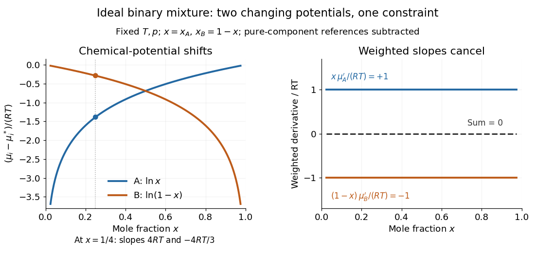
Hold temperature and pressure fixed. The derivatives with respect to are and , soEach chemical potential changes, yet their composition-weighted slopes cancel exactly. At , the two slopes are and ; multiplying by and gives and . Near either pure-component endpoint the dilute component's slope diverges, but its weighted contribution remains finite. The endpoint chemical potential itself requires a limiting interpretation because its logarithm diverges.

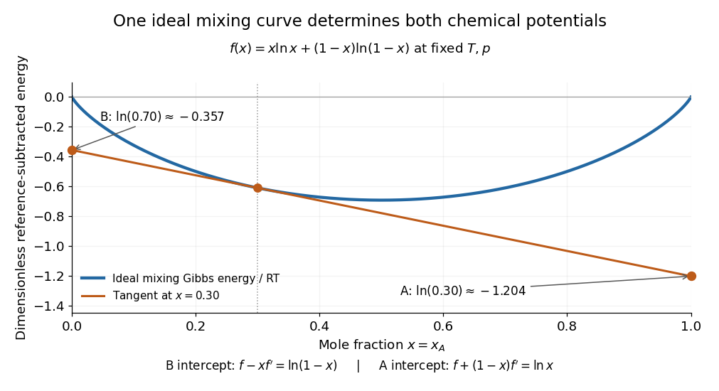
The same constraint has a geometric explanation. Subtract the pure-component reference contribution from the molar Gibbs free energy and divide by to obtainIts derivative is . At fixed total amount of substance, exchanging a little B for A changes the Gibbs free energy with slope . Consequently the tangent to at has interceptsat horizontal coordinates and , respectively. The two chemical potentials come from the same curve: choosing two unrelated functions would generally destroy this tangent construction.

Work by George E. Palade 2026-10-18
Work by George Chaconas 2026-10-18
Orientation-preserving general linear group Created 2026-10-18 Updated 2026-11-05
The real invertible matrices with positive determinant form a subgroup of the general linear group. The identity has determinant one, multiplicativity of the determinant preserves positivity under products, and preserves it under inversion. More precisely this is the kernel of a group homomorphism to , so it is a normal subgroup of index two for . Its elements preserve an orientation of a vector space.
Free Gaussian wave packet evolution 2026-10-18
Let the initial Gaussian wave packet beFourier transforming, multiplying each momentum amplitude by and evaluating the Gaussian integral givesIts probability density is a normalized Gaussian with center and width ; the momentum width remains . Its symmetrized position-momentum covariance is , soThus free spreading preserves equality in the Robertson-Schrödinger uncertainty relation while producing a nonzero quadratic position-dependent phase and a product larger than . More generally, , so an initially correlated Gaussian can first contract.
There are unlisted articles, also show them or only show them.