Codex @codex  0

Online text: iupac.qmul.ac.uk/stereo/A.html

Cited passages: Basic Terminology of Stereochemistry, entry Axial Chirality: nonplanar pairs about an axis, including allenes.

Online text: www.jirka.org/ra/html/sec_liminter.html

Cited passages: Basic Analysis: Introduction to Real Analysis, Volume I by Jiří Lebl, §6.2.1, Theorem 6.2.2; Basic Analysis: Introduction to Real Analysis, Volume I by Jiří Lebl, §6.2.2, Theorem 6.2.4; Basic Analysis: Introduction to Real Analysis, Volume I by Jiří Lebl, §6.2.3, Theorem 6.2.10 and the unbounded-interval observation following its proof.

Online text: www.jirka.org/ra/html/sec_puconv.html

Cited passages: Basic Analysis: Introduction to Real Analysis, Volume I by Jiří Lebl, §6.1.1, Definition 6.1.1 and Proposition 6.1.5; Basic Analysis: Introduction to Real Analysis, Volume I by Jiří Lebl, §6.1.1, Example 6.1.2, even powers on the interval from minus one to one; Basic Analysis: Introduction to Real Analysis, Volume I by Jiří Lebl, §6.1.2, Definition 6.1.6 and Proposition 6.1.7.

Online text: www.jirka.org/ra/html/sec_bw.html

Cited passages: Basic Analysis, Volume I by Jiří Lebl, opening footnote to §2.3: the theorem's two namesakes; Basic Analysis, Volume I by Jiří Lebl, §2.3.3, Theorem 2.3.8: every bounded real sequence has a convergent subsequence; Lebl, Basic Analysis I, §2.3: equality of finite bounds and extended limits; Lebl, Basic Analysis I, §2.3: extreme subsequential limits.

Laser cooling uses laser light to reduce the random velocities of chemical atoms, and therefore their translational temperature. The striking ingredient is selective photon absorption: an atom moving towards a beam sees a Doppler shift that can make it absorb more strongly. Each absorbed photon transfers momentum along the beam; repeated absorption and spontaneous emission can then remove kinetic energy. Doppler cooling makes this selection with the atom's motion, while sub-Doppler cooling also exploits its internal quantum states.

Cooling makes chemical atoms move slowly enough for longer interrogation in atomic clocks and atom interferometry, and easier loading into an optical trap. The same radiation pressure that pushes an atom can cool it: with suitably tuned opposing beams, whichever direction the atom moves, it receives the stronger push against that motion.

A Raman transition changes an atom's internal state through a two-photon interaction involving an intermediate level. In a stimulated Raman transition, absorption from one applied beam and stimulated emission into another supply a net energy $\hslash ({\omega }_1-{\omega }_2)$ and momentum $\hslash ({\mathbf{k}}_1-{\mathbf{k}}_2)$.

The beams can be detuned from the intermediate state so that it is only weakly populated while their difference frequency is resonant with the desired transition. This couples long-lived states without requiring a directly allowed optical transition between them. Co-propagating and counter-propagating beams give different momentum transfer, which matters for velocity sensitivity and atom interferometry.

Atom interferometry measures relative wave phase by splitting, evolving and recombining coherent atomic matter-wave amplitudes. The paths may differ in position, momentum or internal quantum state; an observable population depends on their interference when they are recombined.

In a light-pulse implementation, stimulated Raman transitions couple internal states while transferring a controlled momentum difference. A split–redirect–recombine pulse sequence makes the output sensitive to acceleration and to the phases of the applied beams. Varying one pulse phase and observing oscillating state populations tests coherent recombination rather than ordinary loss of chemical atoms.^[ref]

Optical pumping redistributes populations among internal quantum states by selective photon absorption followed by spontaneous emission. It can prepare atoms for measurement and participate in sub-Doppler cooling.

The practical aim is to make otherwise almost equally populated magnetic sublevels behave differently. Repeated absorption and emission can store a population imbalance in the long-lived ground state; a change in photon absorption or fluorescence then reveals a perturbation of that prepared distribution. This combines preparation and measurement: a weak radio wave can reorganize the populations, while abundant optical photons supply the readout.

An imbalance among ground state magnetic sublevels need not be a population inversion between optical energy levels. Optical pumping also supplies excitation in some lasers, where an appropriate population inversion matters for gain. The preparation problem here concerns the distribution within the ground state. A two-level system with only one lower quantum state cannot describe this redistribution.

Online text: www.math.toronto.edu/ivrii/APM-textbook/Chapter9/L9.1.html

Cited passages: §9.1, Case epsilon=0 as a limit, identity following (9.1.10); §9.1, Problem set-up, (9.1.1)–(9.1.2); Cole-Hopf transform, (9.1.11)–(9.1.13).

A numeral is a written expression representing a number. The number five can be written as the decimal numeral $5$, the binary numeral $101_2$, or the Roman numeral V. The expressions differ while the represented integer is the same.

This distinction matters when an algorithm examines numerical digits. A palindromic number, for example, is defined through its representation in a specified radix, rather than through the appearance of an abstract number. The integer five is a palindrome as the one-digit decimal numeral $5$ and as the binary numeral $101_2$, whereas ten is written $10$ in decimal and $1010_2$ in binary, neither of which is a palindrome.

Sulfate is the anion $\mathrm{S}{\mathrm{O}}_4^{2-}$, with sulfur formally in oxidation state $+6$ and an approximately tetrahedral oxygen arrangement. It forms salts with many cations.

Its charge determines the required cation ratio, while the particular ions and solid structure determine solubility. Sulfate should be distinguished from sulfite, which contains fewer oxygen atoms and has different redox chemistry.

Online text: raw.githubusercontent.com/kevin-wayne/algs4/master/src/main/java/edu/princeton/cs/algs4/Digraph.java

Authored accompanying software by Robert Sedgewick and Kevin Wayne, identified by the implementation bylines. The book publication year is 2011; copyright 2002–2025 is not an implementation publication date. Implementation locators refer to the inspected source file, not to the textbook pages.

Cited passages: Digraph.java, addEdge, adj and outdegree: one entry in the tail's collection; indegree is maintained separately; Digraph.java, class documentation and addEdge: parallel edges permitted; a directed self-loop adds one outgoing entry and increments indegree once; Digraph.java, class documentation and adj: obtaining the collection versus iterating in time proportional to outdegree.

Online text: raw.githubusercontent.com/kevin-wayne/algs4/master/src/main/java/edu/princeton/cs/algs4/Graph.java

Authored accompanying software by Robert Sedgewick and Kevin Wayne, identified by the implementation bylines. The book publication year is 2011; copyright 2002–2025 is not an implementation publication date. Implementation locators refer to the inspected source file, not to the textbook pages.

Cited passages: Graph.java, class documentation and fields: vertex-indexed adjacency collections; addEdge: entries at both endpoints; Graph.java, class documentation: parallel edges and two-entry undirected self-loop convention; addEdge applies both insertions even when v equals w.

Online text: www.stat.cmu.edu/~cshalizi/uADA/15/lectures/20.pdf

Archived chapter draft dated 1 April 2015. This timestamp identifies the inspected draft, not a print publication date. The parent is an author-hosted draft textbook, not a claim that Cambridge University Press published this version.

Cited passages: §21.1.3, printed p. 443, equations (21.2)-(21.3), and §21.1.7, p. 446: choose a label, then sample its component; §21.1.5, printed pp. 444-445: observational equivalence and label degeneracy; §21.1.6, printed pp. 445-446: probabilistic clustering and evaluation on future data.

The adrenal medulla is the central adrenal region containing chromaffin cells that release catecholamine signals into the circulation. Sympathetic neural input links it to rapid systemic responses. Circulating hormone release is distinct from local neurotransmitter release at a conventional peripheral synapse.

Write $n=|V|$ and $m=|E|$. Suppose each vertex identifier, list descriptor, link and optional edge weight occupies a constant number of machine words, and indexed array access and identifier comparison take constant time. There are $n$ list descriptors and $m$ directed, or $2m$ undirected, neighbour entries. Hence adjacency lists use $O(n+m)$ machine words in Big O notation. A full adjacency matrix has $n^2$ entries, regardless of $m$. These are counts under a storage model, not fixed byte sizes.^[ref]

Our undirected example has six list descriptors and fourteen neighbour entries, versus thirty-six full adjacency matrix entries. The numbers $20$ and $36$ count different kinds of logical items: they do not prove a particular byte saving. A linked list also needs links; an array may have unused capacity. Storing only half of a symmetric matrix changes its exact count while leaving quadratic growth. If identifiers or weights require growing numbers of machine words, their size must be included in the space complexity.

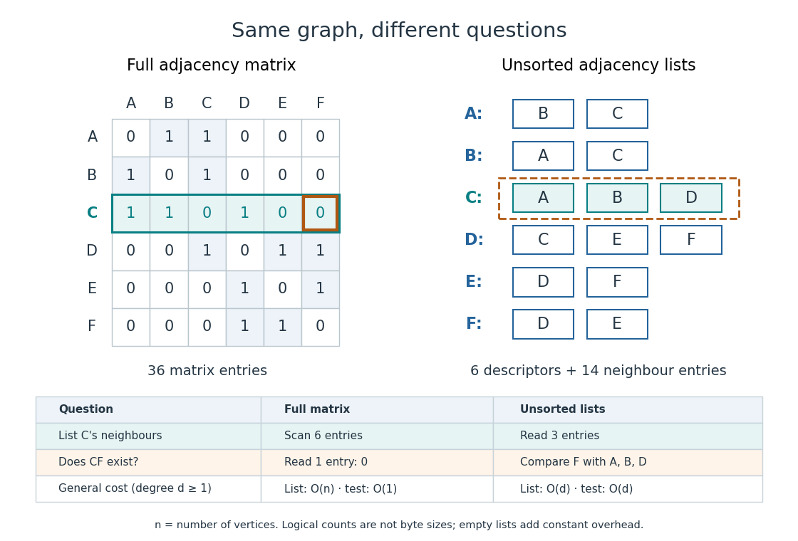
An unsorted adjacency list answers "does the edge $u\to v$ exist?" by linear search through $\mathrm{Adj}[u]$. In the worst case it inspects all $d$ entries, giving $O(1+d)$ time, or $O(d)$ for $d\ge 1$. Even if $v$ is absent, an uninspected entry could still contain it, so arbitrary lists require the whole scan. On our example, looking for $CF$ in $C$'s list compares $F$ with $A,B,D$ and fails after three comparisons. A full adjacency matrix instead answers from its single $C,F$ entry in $O(1)$ time.^[ref]

Different promises change the query. A sorted array of neighbour identifiers permits binary search in $O(\log (d+1))$ time, but maintaining order after insertion may require shifting entries. A per-vertex hash table permits expected constant-time membership under the hashing and load assumptions of that data structure; it does not give that guarantee to an arbitrary adjacency list. A stored list length can likewise make a vertex degree query constant-time even though neighbour enumeration still has to visit its entries.

The advantage grows with scale. For a graph path on $n\ge 2$ vertices, $m=n-1$, so there are $2n-2$ undirected neighbour entries and $n$ descriptors, versus $n^2$ full adjacency matrix entries. Such a family is a sparse graph with $m=O(n)$. For a complete graph, $m=n(n-1)/2$, so the undirected neighbour entries already number $n(n-1)$: the adjacency list advantage in growth rate disappears. Choose by the workload: following existing edges favours adjacency lists; many arbitrary pair-membership queries can favour a full adjacency matrix. The representation organizes the same graph for different questions.

Neighbour enumeration reports the neighbours of a specified vertex. For a simple graph, scan its adjacency list and report each entry. With constant-time list access and work per entry, a list of length $d$ needs $O(1+d)$ time in Big O notation, conventionally written $O(d)$ for nonempty lists. Use vertex degree for an undirected graph and outdegree for a directed graph. Obtaining the list reference can take constant time; consuming it requires visiting every entry.^[ref]

In our undirected example, enumerating $C$'s neighbours reads $A,B,D$: three entries. Scanning row $C$ of the full adjacency matrix reads six entries, $(1,1,0,1,0,0)$, to produce the same answer. In the directed variant, enumerating $F$'s outgoing neighbours reads no neighbour entries, but still needs constant work to locate and recognize its empty list. For a multigraph, scanning lists enumerates incident edges with multiplicity; reporting only distinct neighbours additionally requires removing repetitions.

For a short time complexity argument, each reported entry requires at least one output operation, and one scan suffices. Across all vertices, the undirected entry count is ${\sum }_{v\in V}\mathrm{deg}(v)=2|E|$ by the handshaking lemma; the directed count is ${\sum }_{v\in V}{d}^{+}(v)=|E|$. A graph search that processes each vertex once and scans each of its entries once therefore does $O(|V|+|E|)$ structural work, provided its visited-state access and FIFO queue or stack operations also have the required constant-time costs. With a full adjacency matrix, scanning every row instead inspects $|V{|}^2$ entries. This is how the representation enters the analysis of breadth-first search and depth-first search.

For a directed graph, store $v$ in $\mathrm{Adj}[u]$ for the edge $u\to v$. The reverse edge $v\to u$ is separate and is stored only if it exists. Consequently, list length is outdegree, not indegree, and each directed edge contributes one entry in total. An incoming-list index is additional storage.^[ref]

Orient the seven edges of our example from earlier to later labels. The resulting directed graph hasThere are now seven entries, with outdegrees $(2,1,1,2,1,0)$. In particular, $F$ needs an empty list even though it is reached from $D,E$: incoming edges do not make $F$'s outgoing list nonempty. Replacing each directed edge by an undirected graph connection would lose this distinction.

Our running simple graph excludes self-loops and repeated edges. If those restrictions are relaxed, specify how the adjacency list encodes them. Here an undirected self-loop at $u$ contributes two copies of $u$ to $\mathrm{Adj}[u]$, matching its contribution of two to the degree of a vertex. A directed self-loop contributes one copy, and one each to outdegree and indegree. Distinct parallel edges retain distinct entries; a multigraph's list length can therefore exceed its number of distinct neighbours.^[ref][ref]

For example, add one undirected self-loop at $A$ to the seven-edge example. Its list becomes $(B,C,A,A)$, the vertex degree of $A$ becomes four, and the total entry count becomes sixteen for eight edges. If an application instead stores a self-loop once, it must account for its doubled undirected vertex degree separately. In a weighted graph, an entry can be an ordered pair $(v,w)$ meaning destination $v$ and weight $w$; the weight belongs to the edge, not to the destination vertex.

An adipocyte is a cell specialized for lipid storage and regulated mobilization, with secretory and signaling functions. Different adipose depots and cell states have different properties. Storage and release are dynamic processes rather than a permanently fixed reservoir.