
Work by Addgene 2026-10-14
Stack machine Created 2026-10-14 Updated 2026-10-31
Stereochemical sequence rule 2026-10-14
Stereochemical sequence rules rank substituents for R and S configuration. Compare the directly attached chemical atoms by atomic number first, then resolve ties by comparing successive shells at the first difference. Isotopes and multiple chemical bonds require additional rules. This ranking convention does not involve optical rotation.[ref]
R and S configuration 2026-10-14
For a tetrahedral stereocenter, rank its four substituents using stereochemical sequence rules. With lowest-priority group pointing away, a clockwise sequence is and a counterclockwise sequence is . Looking from the other side reverses the apparent sequence, so the viewing condition is essential. The geometric letters A/B/C/D in the tetrahedral mirror-image test carry no assigned priority. Neither nor determines positive or negative optical rotation.[ref]
5.5 Sequence Rules for Specifying Configuration. McMurry, Organic Chemistry, §5.5, Figure 5.8 and discussion after Figure 5.10
Voltage divider teaching experiment 2026-10-14
Southern Illinois University's ET 304A guide, Lab 4: Voltage Measurements and Meter Loading Effects, documents an instructive test: build equal-arm voltage dividers on a supply, then measure across the lower arm with a digital multimeter, analog multimeter, and oscilloscope. Starting with two resistors, repeat with equal pairs from to . It requires separate recorded readings, unloaded predictions, and predictions including each instrument's input electrical resistance. The guide obtains meter resistances from specification sheets and scope resistance from the input-panel marking. Equal ratios control the unloaded target while changing susceptibility to voltmeter loading. The provided tables are blank: the guide specifies a procedure, not measured outcomes.[ref]
Preparation and accuracy checks are made concrete by Berkeley's Lab 1: Introductory Experiments and Linear Circuits I. Its different divider uses nominal and resistors and a supply on a breadboard. Measure isolated resistors first, record actual supply voltage, recalculate with these measured values, then record the junction voltage with the digital multimeter. It explicitly compares actual values with resistor tolerance and the final voltage with a range-dependent accuracy bound from the instrument manual. This is an uncertainty check, not an independent measurement calibration.[ref]
For a controlled comparison, additionally record the selected instrument range, probe factor, and input coupling; connect each instrument separately to the same electrical reference potential, and monitor the input rather than treating the supply label as an exact voltage. These are proposed controls for interpreting the documented procedures. A voltage indication and a resistance indication from the same digital multimeter do not independently validate its measurement calibration; a traceable reference comparison would be needed for that. Resistor tolerance describes component variation, while measurement uncertainty describes what is known about measured values. Using nominal arms alone can confuse mismatch with loading: equal nominal arms each within one-percent tolerance can give unloaded ratios from to .
The inference to test is specific: once actual arm values, input voltage, and meter input electrical resistance are accounted for, the readout should approach the loaded voltage divider prediction within the remaining measurement uncertainty. A discrepancy can instead reflect contacts, changing temperature, source droop, or an input that is not a fixed passive resistor. A source with positive series electrical resistance can be modeled by replacing with only when denotes its ideal internal voltage; when the actual voltage across the divider is measured, that terminal value is already . During settling, or with appreciable input capacitance and changing signals, the steady direct current calculation is insufficient. Neither institutional procedure supplies measured values for the original example above.
Voltage divider loading error 2026-10-14
For and , define the fractional shortfall in output magnitude from the unloaded value byThis is a loading bias relative to the unloaded target, not the uncertainty of an instrument's measurement of the connected circuit. The equality with the signed ratio also holds for negative , because the output retains its sign. The Thévenin resistance summarizes the divider's susceptibility: the relevant comparison is , not merely a large absolute .
Set and . ThenThe derivative proves that increasing the load electrical resistance always reduces this error. For equal divider arms, : gives , gives , and gives . Thus a “ten times the lower resistor” rule does not guarantee one-percent agreement with the unloaded target.
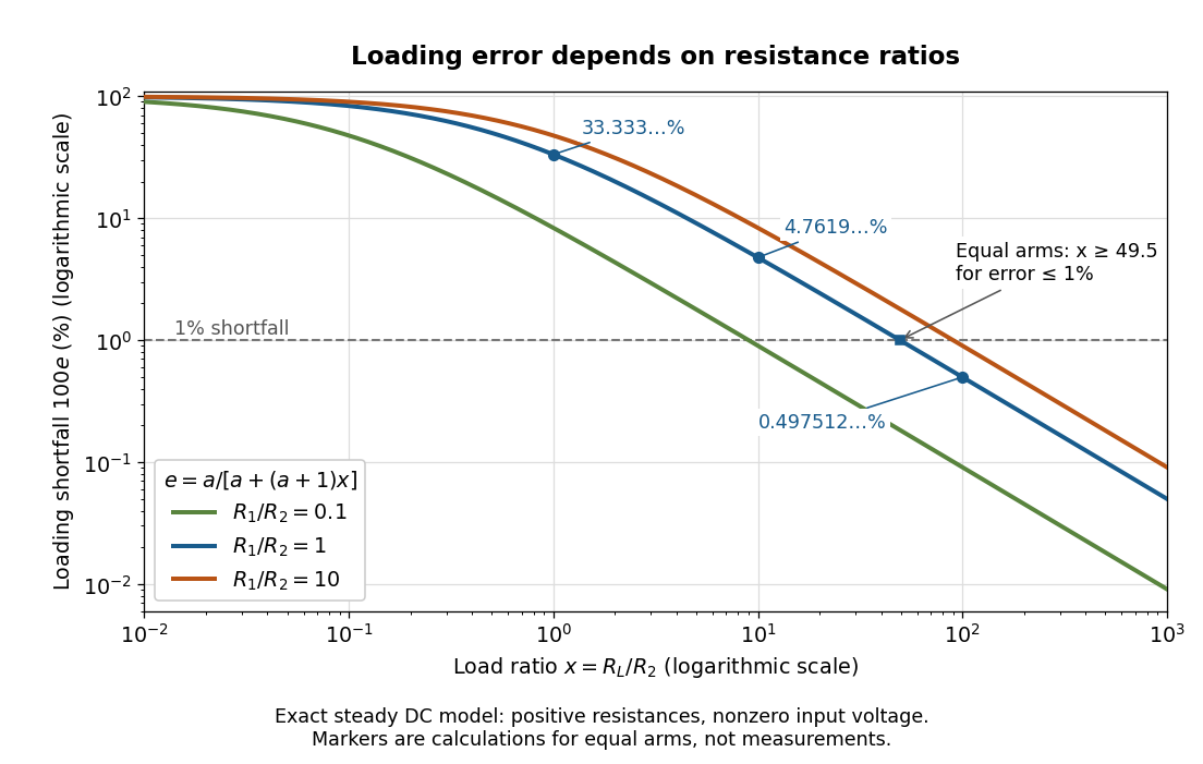
Fractional loading error falls continuously as the load resistance grows relative to the lower divider arm
. Original exact resistance-only predictions for three ratios. The logarithmic axes show the equal-arm examples , including the stipulated load on a lower arm. No points represent measurements. Source. Details.
A quantitative design requirement follows without a rule of thumb. For a specified ,For equal arms, , so one-percent loading error requires . Reducing both divider electrical resistances reduces loading but increases unloaded supply electric current and Joule heating: . The stipulated equal-arm example dissipates in total when unloaded. This tradeoff explains why the ratio alone does not determine a useful divider.
Loaded voltage divider 2026-10-14
Connect a passive electrical load of electrical resistance from the junction to the reference. In the steady direct current model, and share the same electric potential difference and are connected in parallel. Their equivalent electrical resistance isThis is the replacement required when a voltmeter is connected across . The inspected teaching guide explicitly models the meter this way.[ref]
The Kirchhoff's current law proof makes the changed assumption visible:The upper resistor carries the sum of the lower and load electric currents, so the two original resistors no longer have equal electric currents. In the stipulated example, , the upper current is , and each lower branch carries .
For a digital multimeter used as a voltmeter, let its input electrical resistance on the selected voltage range be . With no other load, set ; if an intended load is also present, use in place of . Two instruments connected simultaneously add two branches. Their ideal indicated value equals the voltage of this altered circuit; voltmeter loading can exist even with perfect measurement calibration. Real readout additionally has measurement uncertainty, offsets, and finite resolution. Consult the actual range and input specifications rather than assigning every digital multimeter the same .
For an oscilloscope, the resistance-only model applies to settled direct current with a compatible input coupling setting. The oscilloscope input and cable also have capacitance; changing signals can therefore have loading that depends on frequency. A probe changes the impedance seen at its tip and the relation between tip voltage and displayed voltage; use the probe-and-input combination's specification and attenuation setting. NJIT's guide models the parallel electrical resistance and capacitance and adjusts probe compensation with a square-wave readout.[ref]
Lab 7: Input Impedance of an Oscilloscope and the Scope Probe, NJIT ECE 291. Lab 7: Input Impedance of an Oscilloscope and the Scope Probe, Introduction, Figure 5 and probe adjustment; Laboratory §1(a)–(c)
Thévenin resistance 2026-10-14
The negative slope of the Thévenin terminal response with delivered electric current . Thévenin source suppression determines it from the ratio of test voltage to entering test electric current. It need not represent a physical positive resistor inside the original network.
Thévenin measurement experiment 2026-10-14
An authored teaching experiment uses an adjustable steady-voltage supply, a digital multimeter, fixed resistors, and a potentiometer or resistance decade box. Its original circuit uses a supply and , , and resistors; the student compares and electrical loads. The readout is load voltage, recorded against prediction and deviation. The student then removes the electrical load to measure the open-circuit voltage, disconnects the supply and substitutes a wire to measure the Thévenin resistance with the multimeter's resistance mode, and restores the supply for an independent method: adjust the variable electrical load until the voltmeter reads half the unloaded voltage. Finally the student builds the equivalent and repeats both load measurements. Its tables are blank recording forms, not reported observations. [ref]
Laboratory Manual for DC Electrical Circuit Analysis by James M. Fiore. Laboratory Manual for DC Electrical Circuit Analysis by James M. Fiore, version 1.4.3, experiment 11, printed pp. 52–55: Equipment, Procedure 1–10, Tables 11.1–11.3
The half-voltage inference assumes negligible voltmeter loading and positive . A finite voltmeter input electrical resistance actually gives an apparent unloaded readingWhen the same voltmeter remains connected across a variable electrical load , the network sees . Setting its reading to , rather than to the true , givesThus the uncorrected half-reading method underestimates positive . In the original example, a stipulated gives and half-reading load , instead of . These are model predictions for a deliberately loading meter, not the specification or observed readout of the source experiment's instrument.
Finite readings can also estimate the terminal line without a physical short. For two distinct load settings with corrected delivered electric currents and terminal voltages ,If the voltmeter remains across each electrical load, the delivered electric current is , including the meter branch. Omitting it biases the inferred slope.
Useful additional controls are to measure each resistor separately before assembly, verify terminal polarity, repeat an earlier load setting to detect supply drift, and compare a third setting with the inferred Thévenin terminal response. These are proposed controls, not reported outcomes of the source experiment. Closely spaced electric currents make the slope estimate sensitive to voltage resolution and measurement error; widely separated settings may trigger source current limiting or Joule heating that changes electrical resistance. Lead and contact electrical resistance, meter input uncertainty and rounding limit the inference. An ohmmeter injects its own test electric current; its reading on a powered network is not the suppressed-network ratio. Measurements with independent sources physically removed do not characterize an active dependent electrical source whose control or supply has also been disconnected.
Thévenin load response 2026-10-14
A positive resistive electrical load obeys Ohm's law, . Its resistive load line intersects the Thévenin terminal response atprovided . For the Thévenin divider example, gives and ; gives and . At , the voltage is , half the open-circuit voltage.
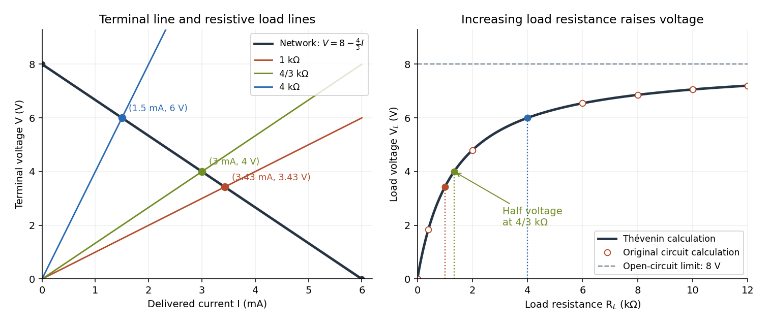

For this positive , increasing reduces the drawn electric current and raises toward . This explains voltmeter loading: a voltmeter itself is an electrical load. The equivalence also applies to a nonlinear electrical load through intersection with its terminal relation, but an arbitrary load need not give a unique operating point. If negative cancels positive , the displayed formula is singular; a real active circuit's limits and dynamics must then be considered.
Thévenin source suppression 2026-10-14
To determine the Thévenin resistance, remove the external electrical load and set each independent electrical source to zero in the circuit model. A zero ideal voltage source enforces zero electric potential difference, so replace it by a short connection. A zero ideal current source enforces zero electric current, so replace it by an open connection. Retain every resistor, including any explicitly modeled supply electrical resistance. Turning an actual power supply's front-panel control to zero is not evidence that it physically becomes an ideal wire.
Retain every dependent electrical source and its controlling variable: its response to an electrical test source is part of the network's electrical resistance. Impose terminal voltage with an electrical test source and calculate entering the suppressed network at . For a nonzero test yielding a finite ratio,Alternatively inject a known entering electric current and solve for . The test electric current is opposite to the delivered-current convention of the original Thévenin terminal response. [ref]
Thevenin and Norton Equivalents, University of Houston teaching notes. Thevenin and Norton Equivalents, pp. 5–7, “Test Source Method for RTH” and Notes: suppress independent sources, retain dependent sources
For an original illustration, put a positive resistor across and a dependent electrical source in parallel that injects electric current from toward , where has units of electrical conductance. Its control is the same terminal voltage . Kirchhoff's current law givesWith and , a test draws , giving . Removing the dependent electrical source would falsely give . With , the model instead has ; with it draws zero test electric current for any imposed voltage and has no finite ratio. An active physical realization requires a supply and has a limited operating range.
For a finite nonzero and a well-defined short-circuit response, . Thus is usable when . A source-free positive resistor has both and , so this quotient cannot reveal its electrical resistance; an electrical test source can.
Thévenin divider example 2026-10-14
In the pictured original linear resistive circuit, the ideal voltage source keeps its upper node at relative to . Let connect that node to , and connect to . With the external electrical load removed, the voltage divider givesTo find the Thévenin resistance, Thévenin source suppression replaces the ideal voltage source by a wire. Both resistors now join to in parallel, givingThis is the electrical resistance looking into the original network with its independent electrical source suppressed; the external electrical load is excluded.
An independent check uses Kirchhoff's current law at , without suppressing anything:The Thévenin terminal response thus follows directly from the original topology. Shorting to in this ideal calculation gives : the lower resistor has zero voltage and the upper resistor limits the electric current. All numerical values here and in the figures are stipulated model values, not laboratory data.
Thévenin terminal response 2026-10-14
With the passive sign convention applied to the network, its entering electric current is , and the same relation becomes . The electrical load uses the passive sign convention with entering electric current , so it absorbs power . A positive delivered electric current therefore produces a voltage drop for positive ; changing the reference direction without changing the equation would give the wrong sign.
The reason is linearity of Ohm's law, Kirchhoff's current law, Kirchhoff's voltage law, and the constitutive relations of any linear dependent electrical sources. Solve once at with the independent electrical sources present. Subtract this solution from a solution with prescribed delivered electric current : the fixed independent electrical sources cancel, leaving a homogeneous linear network whose terminal voltage change is proportional to . This is a short superposition principle argument for an affine function; the fixed offset need not vanish.
The qualification about a well-defined response matters. An ideal voltage source alone has . An ideal nonzero current source alone constrains and does not have a finite open-circuit voltage or a representation with finite coefficients. Linear dependent electrical sources can give negative resistance, and singular ideal networks may fail to have a unique finite response. Neither a finite nor a strictly positive passive follows merely from calling an electrical circuit linear. [ref]
Thevenin and Norton Equivalents, University of Houston teaching notes. Thevenin and Norton Equivalents, p. 11, “On a Negative Thevenin Equivalent Resistance”: dependent-source models can have negative equivalent resistance
Abstract machine 2026-10-14
An abstract machine specifies a computational state and rules for advancing that state without requiring one particular physical implementation. A Turing machine and a stack machine give different ways to organize the state and its transitions.
Decibel 2026-10-14
Substituent 2026-10-14
A substituent is an attached chemical atom or group considered relative to a chosen molecular framework. Testing whether two substituents are identical may require comparing their full chemical bond connectivity and stereochemistry.
Conformational isomerism 2026-10-14
Conformational isomerism concerns spatial arrangements interconverted by internal motion, such as turning about a single chemical bond. Moving the entire molecule or applying a rotation changes its position or viewing direction, not its internal arrangement.
Absolute configuration 2026-10-14
Absolute configuration records a spatial arrangement without leaving its handedness relative to its mirror unspecified. R and S configuration is one naming convention; optical rotation is a measured response.
Stereoisomer 2026-10-14
Stereoisomers have the same chemical bond connectivity but different spatial arrangements. A mirror pair of distinct stereoisomers comprises enantiomers; diastereomers have no mirror-pair relation.
Spreadsheet tabular model 2026-10-14
A spreadsheet tabular model assigns a consistent meaning to each row and column. For an original example, let rows 2–4 describe three items, with quantity in column
A, unit price in column B, subtotal in column C, and total including tax in column D. Put the single shared tax rate in F1. The chosen rate is an illustrative assumption. Quantities, unit prices and F1 are inputs; columns C and D hold spreadsheet formulas and display their computed values as outputs.Enter decimal inputs
2.5, 1.75, 4.5 for the unit prices and 0.2 for the tax rate. The following table expresses those values as exact fractions so that the arithmetic is easy to check. It does not require typing a fraction into an input spreadsheet cell or assume that all software calculates with exact rational numbers.Start with
C2 containing =A2*B2 and D2 containing =C2*(1+$F$1). Here * requests multiplication, and 1+$F$1 adds the tax fraction to one. Copy these two spreadsheet formulas down into rows 3 and 4, a fill operation. The relative spreadsheet references change with the destination row: C3 becomes =A3*B3 and D3 becomes =C3*(1+$F$1); C4 becomes =A4*B4 and D4 becomes =C4*(1+$F$1). The absolute spreadsheet reference $F$1 continues to read the shared rate. Copying spreadsheet formulas adjusts relative coordinates while retaining absolute coordinates. [ref]Addresses and References, Absolute and Relative, LibreOffice Help. Addresses and References, Absolute and Relative: Relative Addressing; Absolute Addressing; When to Use Relative and Absolute References, final two paragraphs
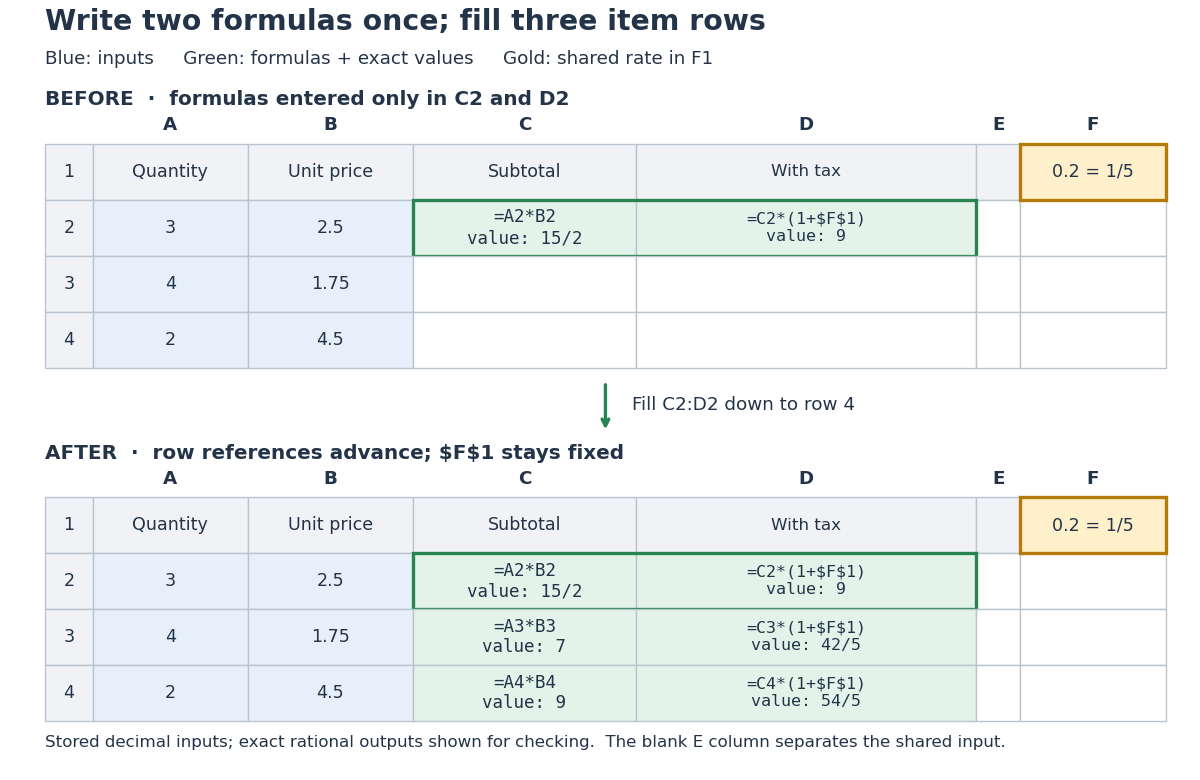
Original three-row spreadsheet tabular model before and after filling two spreadsheet formulas, with a shared absolute spreadsheet reference
. Details. 
The same mathematical expression applies to every item. Writing for quantity, for unit price and for the shared tax rate givesFor row 2, the exact arithmetic is . The subtotals add to , so the totals add to , agreeing with . The spreadsheet formulas encode the relationship; the displayed numbers are its results for these particular inputs.
This separation is useful for forecasting and sensitivity analysis. Keeping quantities and unit prices fixed while changing only
F1 from to gives exact totals , , and . More generally, a rate change changes each total byThis follows by expanding the two mathematical expressions and cancelling . Here , so the increases are , , and , adding to . One shared input makes the assumption visible and consistent across all rows. Overwriting a computed total with a number would instead remove that spreadsheet formula; its value would cease to follow the model when the rate changes.// Target: computer-science.bigb
There are unlisted articles, also show them or only show them.