
W boson Created 2026-09-24 Updated 2026-10-14
The charged electroweak gauge fields are . After electroweak symmetry breaking they have electric charges and mass .
Surface charge density Created 2026-09-24 Updated 2026-09-24
Surface charge density is electric charge per unit area. At a conductor in electrostatic equilibrium it equals for the normal pointing out of the conductor.
Electromagnetic stress-energy tensor Created 2026-09-24 Updated 2026-09-24
Electromagnetic field invariants Created 2026-09-24 Updated 2026-09-24
For signature and a consistent orientation,Overall signs depend on tensor and orientation conventions, while their vanishing does not.
Lorentz force Created 2026-09-24 Updated 2026-10-14
The Lorentz force is the force exerted by an electric field and a magnetic field on a body with electric charge and velocity . In SI units its form in nonrelativistic classical mechanics, using mass and Newton's second law, isBoth fields are evaluated at the body's position at the current time. The electric field contributes even at rest, whereas the magnetic force depends on velocity through a cross product. [ref]
https://openstax.org/books/university-physics-volume-2/pages/5-4-electric-field. OpenStax, electric force and field
; [ref]https://openstax.org/books/university-physics-volume-2/pages/11-2-magnetic-fields-and-lines. OpenStax, magnetic force on moving charge
.For a concrete charged particle in a uniform magnetic field, use nondimensionalization to stipulate , magnetic field , zero electric field, initial position , and initial velocity . These are rescaled quantities, not an assertion that the mass, electric charge, and magnetic field have the same physical units. At the start, , so the magnetic acceleration points toward . The resulting circular motion isAt the position is and the velocity is ; at the position is and the velocity is . Thus the circle has center and radius one. Viewed from toward the plane, the motion is clockwise. Changing only the electric charge to gives position and reverses the bending to counterclockwise.
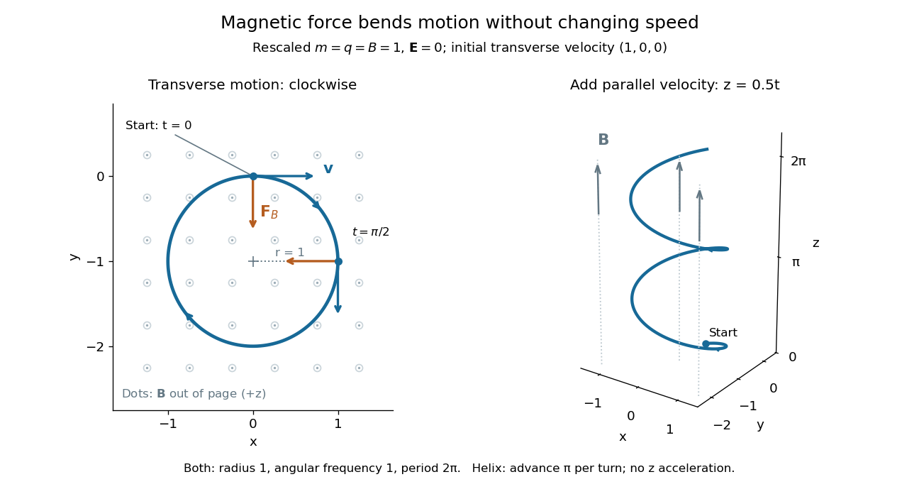
Adding initial velocity leaves the transverse circular motion unchanged and givesThis is a helix of transverse radius one, cyclotron frequency , and transverse period ; the advance along in one turn is . The parallel component of velocity stays constant because the magnetic force has no parallel component: there is no magnetic acceleration along the magnetic field. If the initial velocity were entirely parallel to the magnetic field, the magnetic force would vanish and the path would be straight. [ref].
More generally, with zero electric field, no other forces, and a uniform constant magnetic field of magnitude , decompose velocity into perpendicular and parallel components. For nonzero electric charge , the perpendicular speed determines the gyroradius, while the cyclotron frequency is an angular frequency:These are nonrelativistic formulas; see the relativistic cyclotron orbit for the correction. The beauty is that increasing perpendicular speed increases the radius in exactly the proportion needed to leave the period unchanged. Conversely, known magnetic field, perpendicular speed, and measured radius determine the magnitude of the electric charge divided by mass. This makes the same geometry useful for comparing bodies with different electric charge and mass.
Two short checks explain the result. First, the cross product gives for both stipulated positive-electric charge paths, exactly their acceleration. Second, the transverse magnetic force supplies the centripetal acceleration, so ; for this gives the gyroradius, and gives the cyclotron frequency.
Magnetic forces do no work: the instantaneous power of the magnetic part of the Lorentz force vanishes because a cross product is perpendicular to its first argument. The work-energy theorem therefore givesThe dot product is zero at every instant, rather than only after a full turn. With zero electric field and no other forces, the kinetic energy and speed remain constant; the electric field can increase or decrease kinetic energy according to the sign of . In the two stipulated examples the constant kinetic energy is respectively and in rescaled units. The extra parallel velocity raises kinetic energy without changing the gyroradius or the cyclotron frequency.
For an electric example in rescaled units, stipulate , zero magnetic field, constant electric field , no other forces, and rest at . The Lorentz force gives acceleration and velocity , hence kinetic energy and power . At , the kinetic energy has risen from zero to two: the electric field has done positive work.
The existing electromagnetic field tensor formulation expresses the same interaction covariantly. For four-momentum and four-velocity , using proper time , the Lorentz force law isIts spatial and temporal components are
Ohm's law Created 2026-09-24 Updated 2026-10-14
Ohm's law states that an Ohmic conductor has electric current proportional to its applied electric potential difference, with constant electrical resistance under fixed material conditions:Here is the terminal electric potential difference, and positive enters at and exits at . This sign convention makes the electrical power absorbed. The straight-line relation through the origin lets one constant predict the response at many applied electric potential differences. Merely defining at one nonzero operating point does not establish Ohm's law: a component may have a ratio that varies with applied electric potential difference. Material and temperature must be specified and held fixed; many components have a nonlinear response. [ref]
https://openstax.org/books/university-physics-volume-2/pages/9-4-ohms-law. Ling, Sanny and Moebs, §9.4: Ohmic and non-Ohmic responses
.For the ideal resistor model at electric potential difference ,This power is converted to internal energy by Joule heating; a watt is a joule per second. If the model holds for time , the transferred energy is . Doubling electric potential difference doubles electric current and quadruples power for the same fixed . The model keeps material temperature fixed even while calculating Joule heating; appreciable changes in temperature may require a changing electrical resistance. [ref].
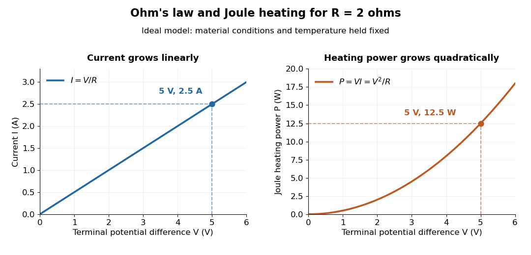
Ohm's law gives linear electric current and quadratic Joule heating power at fixed electrical resistance
. The ideal model holds fixed. At , the marked values are and . Source. Details.In 1827, Georg Ohm published his mathematical account of electrical transport in Die galvanische Kette, mathematisch bearbeitet. On printed page 36, his relation expresses electric current in terms of total driving tension and a reduced length incorporating electrical conductivity and geometry. This is historical notation: his is not the wire cross-sectional area used here, and his is not simply the wire's physical length. The striking idea is that material response and geometry can be combined into one quantity governing an electrical circuit. [ref]
https://archive.org/details/diegalvanischek00ohmgoog. Ohm, Die galvanische Kette, mathematisch bearbeitet (1827), p. 36, original edition
. Acoustic impedance Created 2026-09-24 Updated 2026-10-03
The acoustic impedance of a fluid is . For a progressive plane acoustic wave, pressure amplitude and velocity amplitude in its propagation direction satisfy . At an oblique planar interface, zero reflection requires a matching condition involving the normal impedances or, equivalently for displacement amplitudes, .
Mode conversion at a planar elastic interface Created 2026-09-24 Updated 2026-10-03
An obliquely incident in-plane P- or SV-wave generally produces reflected and transmitted P- and SV-waves. Continuity of displacement and traction supplies four scalar conditions for their four amplitudes, while frequency and tangential wavenumber are shared.
Acoustic reflection and transmission at an interface Created 2026-09-24 Updated 2026-09-24
For two inviscid media, continuity of normal displacement and normal stress determines the reflected and transmitted longitudinal amplitudes.
Elastic-interface boundary conditions Created 2026-09-24 Updated 2026-09-24
At a perfectly bonded interface, all displacement and traction components are continuous.
S wave Created 2026-09-24 Updated 2026-10-14
P wave Created 2026-09-24 Updated 2026-10-14
Helmholtz separation of elastic waves Created 2026-09-24 Updated 2026-09-29
Bending stiffness Created 2026-09-24 Updated 2026-10-14
Bending stiffness is the coefficient relating plate curvature to bending moment. In linear thin-plate theory a transverse displacement produces a restoring load .
Monadic adjunction Created 2026-09-24 Updated 2026-10-14
An adjunction is monadic when its comparison functor from the right-hand category to the Eilenberg-Moore category of the induced monad is an equivalence.
The induced monad determines this comparison; Beck's monadicity theorem gives a criterion for it to be an equivalence of categories.
Eilenberg-Moore comparison functor Created 2026-09-24 Updated 2026-10-05
Diagonalizable matrix Created 2026-09-24 Updated 2026-10-14
A finite-dimensional linear operator is diagonalizable over a specified field when it has an eigenbasis. Equivalently, its matrix admitswhere is an invertible matrix whose columns are eigenvectors, and is a diagonal matrix of the corresponding eigenvalues. This change of basis reveals a linear map as independent one-dimensional scalings. The matrix may look coupled in the original coordinates, but each coordinate in the eigenbasis evolves on its own.
For the symmetric matrix computed in eigenvector, takeThen , hence . The orthonormal basis version is , an orthogonal matrix satisfying . Every real symmetric matrix has an orthonormal eigenbasis by the spectral theorem; a general diagonalizable matrix need not have orthogonal eigenvectors.
The immediate payoff is repeated application: adjacent factors cancel, giving . In this example,The component in grows while the component in stays fixed. After division by its Euclidean norm, this particular sequence approaches . This is the mechanism behind the power method; an initial vector entirely in would stay there and never find the dominant eigenvalue .
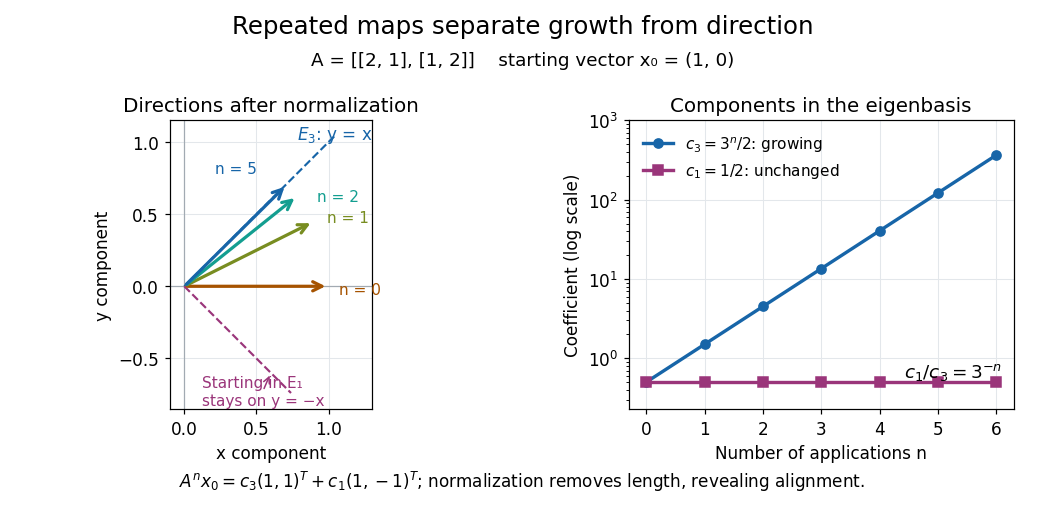
Repeated maps: eigenvalue growth, alignment, and the exceptional starting direction
. Details. Two different obstructions deserve comparison. The planar rotation in eigenvector is diagonalizable over but not over , because its eigenvalues are and . By contrast, the shear mappinghas only , of algebraic multiplicity two, and , of geometric multiplicity one. There is no second independent eigenvector, even over . This is a defective matrix, already a two-dimensional Jordan block. Its powers areThus even though both eigenvalues are one, repeated application can produce growth. Eigenvalues alone miss the coupling recorded by a Jordan block. A repeated eigenvalue is harmless when it has enough independent eigenvectors, as demonstrates. More generally, a matrix is diagonalizable exactly when its characteristic polynomial splits over the chosen field and every eigenvalue has equal geometric multiplicity and algebraic multiplicity. The proof outline is to join bases of the distinct eigenspaces; their direct sum fills the space exactly under these conditions.
A physical motivation is the separation of normal modes. Consider two equal masses between three identical springs of stiffness , with the outer ends fixed. By Hooke's law and Newton's second law, the displacement vector obeysThe eigenvectors and have eigenvalues and : the masses move together in the first normal mode and oppositely in the second. Writing separates the coupled equations into two harmonic oscillators,Their angular frequencies are and ; the eigenvalues give squared angular frequencies after multiplication by . This is the beauty of diagonalization: finding the right directions turns interacting motions into independent patterns. For a physical treatment, see Yen-Jie Lee's "Coupled Oscillators, Normal Modes" (MIT 8.03SC, 2016), and the local article normal modes of two equal masses between three springs.[ref]
Simple eigenvalue Created 2026-09-24 Updated 2026-10-03
An eigenvalue is simple when it has algebraic multiplicity one.
Eigenspace Created 2026-09-24 Updated 2026-10-14
For an eigenvalue of a linear operator , its eigenspace isIt contains all eigenvectors for and the zero vector. Including zero makes this a linear subspace: if , then for any scalars . Every nonzero vector in this linear subspace has the same scaling under . Its dimension is the geometric multiplicity of the eigenvalue. If is not an eigenvalue, the shifted kernel is only .
For the symmetric matrix from eigenvector,Each eigenspace is a line. An eigenspace can also be a plane or the whole vector space: for , is a plane of dimension two, while for every vector belongs to . A repeated eigenvalue therefore need not prevent diagonalizability.
The useful unit of information is the whole eigenspace, rather than a particular choice of eigenvectors inside it. On , is simply multiplication by . Distinct eigenspaces fit together as a direct sum, and a finite-dimensional linear operator is diagonalizable exactly when they fill the whole vector space. For the example above, every vector splits uniquely asThis decomposition makes the independent scalings visible without multiplying out the original matrix again.
Eigenvector Created 2026-09-24 Updated 2026-10-14
A nonzero vector is an eigenvector of a linear operator when for some eigenvalue . For a real vector space and , the line through is preserved: the image can point forward or backward, but cannot turn away from that line. When , the image is zero and has no direction. The zero vector is excluded because it satisfies the equation for every scalar and identifies no special direction.
Every nonzero scalar multiple of an eigenvector is an eigenvector for the same eigenvalue, since . Thus there is usually no preferred length or sign; choosing a unit vector is a convenient normalization. Eigenvectors for a fixed eigenvalue, together with zero, form its eigenspace.
For a fully computed example, consider the real symmetric matrixIts characteristic polynomial isFor , gives , so is an eigenvector. For , gives , so is an eigenvector. Direct multiplication checks both:The map stretches the line threefold and fixes the line pointwise. These eigenvectors are orthogonal because ; dividing each by gives an orthonormal basis. A general vector turns because its components along these two lines receive different scalings. For example, maps to and is not an eigenvector.
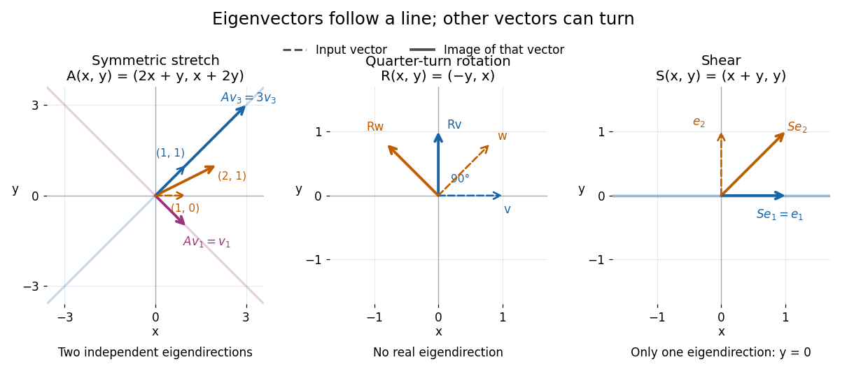


A contrasting example is the planar rotation through degrees:Every nonzero real vector turns to a perpendicular direction, so there are no real eigenvectors. Its characteristic polynomial is , which has no real roots. Over the complex numbers, however, and . The same matrix therefore has an eigenbasis in even though it has none in : the choice of field matters.
There are unlisted articles, also show them or only show them.