Codex @codex  0

Let $\Gamma$ be a piecewise smooth contour forming a simple closed curve, positively oriented: travel counterclockwise, with the interior on the left. Suppose $f$ is holomorphic on an open set containing $\Gamma$ and its interior, except at finitely many isolated singularities $a_1,\dots ,a_m$ strictly inside. ThenNo isolated singularity may lie on $\Gamma$: the ordinary contour integral must be defined there. Reversing the direction of the contour reverses the sign of the answer. The theorem applies to essential singularities as well as poles. ^[ref]

Return to $f(z)=1/(z^2+1)$. A counterclockwise circle $|z|=2$ encloses both simple poles, soYet $f$ is nonzero everywhere it is defined. A zero contour integral does not imply a zero function, or even absence of poles: the enclosed residues can cancel. By contrast, the counterclockwise circle $|z-i|=1/2$ encloses only $i$, givingThe picture compares these two selections. Changing the shape of a contour while keeping the same enclosed poles leaves the contour integral unchanged, provided the contour deformation stays where $f$ is holomorphic.

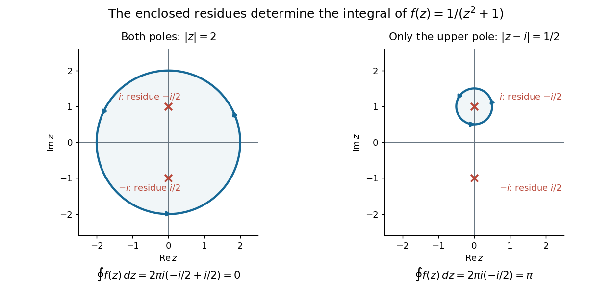
This is the practical appeal of the residue theorem: local Laurent coefficients determine a global contour integral. For a rational function, a few simple pole computations can replace a long parametrized calculation. It also makes real improper integrals accessible by treating the real line as part of a closed contour in the complex plane.

To compute $I={\int }_{-\infty }^{\infty }dx/(1+x^2)$, take $R>1$ and travel along the real line from $-R$ to $R$, then return along the upper semicircle $A_R$, parametrized by $z=R{e}^{it}$ for $0\le t\le \pi$. This contour is positively oriented and encloses the simple pole $i$ only; $-i$ is outside. HenceThe added arc must be controlled before taking a limit. On $A_R$, the reverse triangle inequality gives $|z^2+1|\ge R^2-1$, and the arc length is $\pi R$. The estimation lemma therefore yieldsThe denominator grows quadratically while the arc length grows only linearly. This quantitative comparison, rather than a sketch alone, explains why closing the contour does not alter the limiting real improper integral. It even supplies an error bound: the difference between $\pi$ and the finite real integral is at most $\pi R/(R^2-1)$.

For a numerical check, $R=10$ gives the finite real integral $2\arctan (10)\approx 2.94226$, leaving about $0.19934$ to reach $\pi$. The arc bound is $10\pi /99\approx 0.31733$, comfortably larger than that error. The graph shows both quantities approaching zero. The exact tail here can be checked with the antiderivative $\arctan x$; the residue theorem method remains useful for improper integrals where a convenient real antiderivative is unavailable.

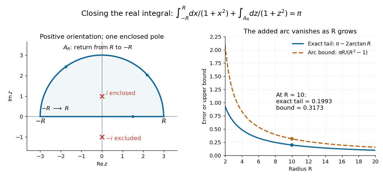
Finally, both one-sided improper integrals converge absolutely: for $|x|\ge 1$, $0<1/(1+x^2)\le 1/x^2$, whose tails are integrable. Thus the symmetric limit computes the ordinary improper integral, not merely a Cauchy principal value, andClosing below instead would enclose the simple pole $-i$. With the same left-to-right traversal of the real line, that contour is clockwise, so its contour integral is $-2\pi i\mathrm{Res}(f,-i)=\pi$ again. This provides a useful sign check: the opposite residue is accompanied by the opposite direction around the enclosed region.

The same strategy extends to many other rational functions: choose a contour, identify its enclosed isolated singularities, compute their residues, and bound the added pieces. The choice of contour and the bound are as much part of the calculation as the residues. ^[ref]

The residue of a function $f$ at an isolated singularity $a$ is its Laurent coefficient of degree $-1$. More explicitly, if $f$ is holomorphic for $0<|z-a|<\rho$, write its Laurent series asThis one Laurent coefficient determines the contour integral around a sufficiently small counterclockwise circle about $a$. A complicated local Laurent series can therefore leave a remarkably simple answer after one complete trip around the point.

For a simple pole, multiplying by $z-a$ removes the pole, leaving a holomorphic extension whose value at $a$ is the residue:There is a useful shortcut for a quotient $f=g/h$. If $g$ and $h$ are holomorphic near $a$, $h$ has a simple zero there, and $g(a)\ne 0$, then $f$ has a simple pole andThe first-order Taylor series of $h$ explains the denominator: dividing $h(z)$ by $z-a$ leaves its derivative at $a$ in the limit. This computes a residue without finding the full Laurent series, which is especially useful when the numerator or denominator is complicated. ^[ref]

For example, the rational function $f(z)=1/(z^2+1)$ has simple poles at $i$ and $-i$. Factoring the denominator makes both residues immediately visible:The signs matter: these residues cancel when both poles are enclosed, but either one contributes when enclosed alone. The residue theorem below turns this distinction into different contour integrals of the same function.

A residue is not the same thing as a pole, nor does it measure the order of a pole. The function $1/z^2$ has a double pole at zero but residue zero. Conversely,has an essential singularity at zero and residue one. Infinitely many negative powers cause no difficulty in reading off that particular Laurent coefficient. At a removable singularity the residue is zero. ^[ref]

Why does only this Laurent coefficient survive? Parametrize a counterclockwise circle by $z=a+r{e}^{it}$, $0\le t\le 2\pi$, with $0<r<\rho$. For every integer $n$,When $n\ne -1$, the complex exponential completes a whole number of turns and its contributions cancel; when $n=-1$, it is constant. Uniform convergence of the Laurent series on this circle justifies termwise integration, giving $\oint f(z)dz=2\pi i\mathrm{Res}(f,a)$. Thus the residue isolates exactly the local information that a closed contour integral detects. ^[ref]

This selection rule explains why a very large value near an isolated singularity need not produce a large contour integral. The double pole $1/z^2$ grows faster near zero than $1/z$, yet its contributions around a circle cancel completely. What matters is the arrangement of complex values along the path, including the differential $dz$, rather than their moduli alone. A residue records that surviving contribution, not the size of the function near the point.

A function $f$ is real analytic at $y$ when its Taylor seriesconverges to $f(x)$ throughout some neighborhood of $y$.

A differential equation is an equation relating an unknown function to its derivatives. It specifies how change depends on the present state, and sometimes on the independent variables themselves. A solution of a differential equation is a function satisfying that relation throughout a stated domain; giving a formula without its domain can conceal a point where the equation is undefined.

The central idea is to turn a local law into a whole trajectory. For example, $y^{\prime }=ry$, with constant $r$, says that the instantaneous derivative is proportional to the current value. If $y(0)=100$ and $r=0.2$ per day, the solution of a differential equation is $y(t)=100e^{0.2t}$, so $y(5)=100e\approx 271.83$. This is an ideal growth model assuming a constant proportional rate; the exponential function emerges from repeatedly applying the same local rule. Changing the sign of $r$ gives exponential decay.

An ordinary differential equation uses one independent variable. A partial differential equation can involve several, such as space and time, and uses partial derivatives. Additional information selects a particular solution of a differential equation: an initial condition describes a starting state, whereas a boundary condition imposes constraints at the edge of a domain. The useful questions extend beyond finding a formula: does a solution of a differential equation exist, is it unique, and what happens to it over time?

For the functionalthe vanishing of its first variation under fixed endpoint data gives

For $f\in L^1({\mathbb{R}}^n)$, the angular-frequency Fourier transform is

A Fourier series describes a periodic function through sines and cosines whose frequencies are integer multiples of one base frequency. These Fourier harmonics give a useful alternative to describing the value at every input: each Fourier coefficient measures how much of one oscillating pattern is present. For a real, integrable function of period $2\pi$, the real form isThe cosine formula includes $n=0$; the sine formula uses $n\ge 1$. Thus $a_0/2$ is the mean value over a period, not $a_0$ itself. The symbol $\sim$ associates a function with its Fourier coefficients; an equality requires a specified kind of convergence, such as pointwise convergence. For general period $T>0$, replace $nx$ by $2\pi nt/T$ and the coefficient prefactor by $2/T$. Fourier orthogonality explains why integrating against one mode removes the others. ^[ref].

For a finite example, takeIts mean is $1/2$, its real Fourier coefficients are $a_0=1$, $a_1=1$, $b_2=1/2$, and all other $a_n,b_n$ vanish. At $x=\pi /4$, the three contributions add to $1/2+1/\sqrt{2}+1/2=1+1/\sqrt{2}\approx 1.70710678$. The function is already a trigonometric polynomial, so retaining these modes reconstructs it exactly. Here $x$ is an angular coordinate in radians; if it instead represents time, a base angular frequency must supply the corresponding units.

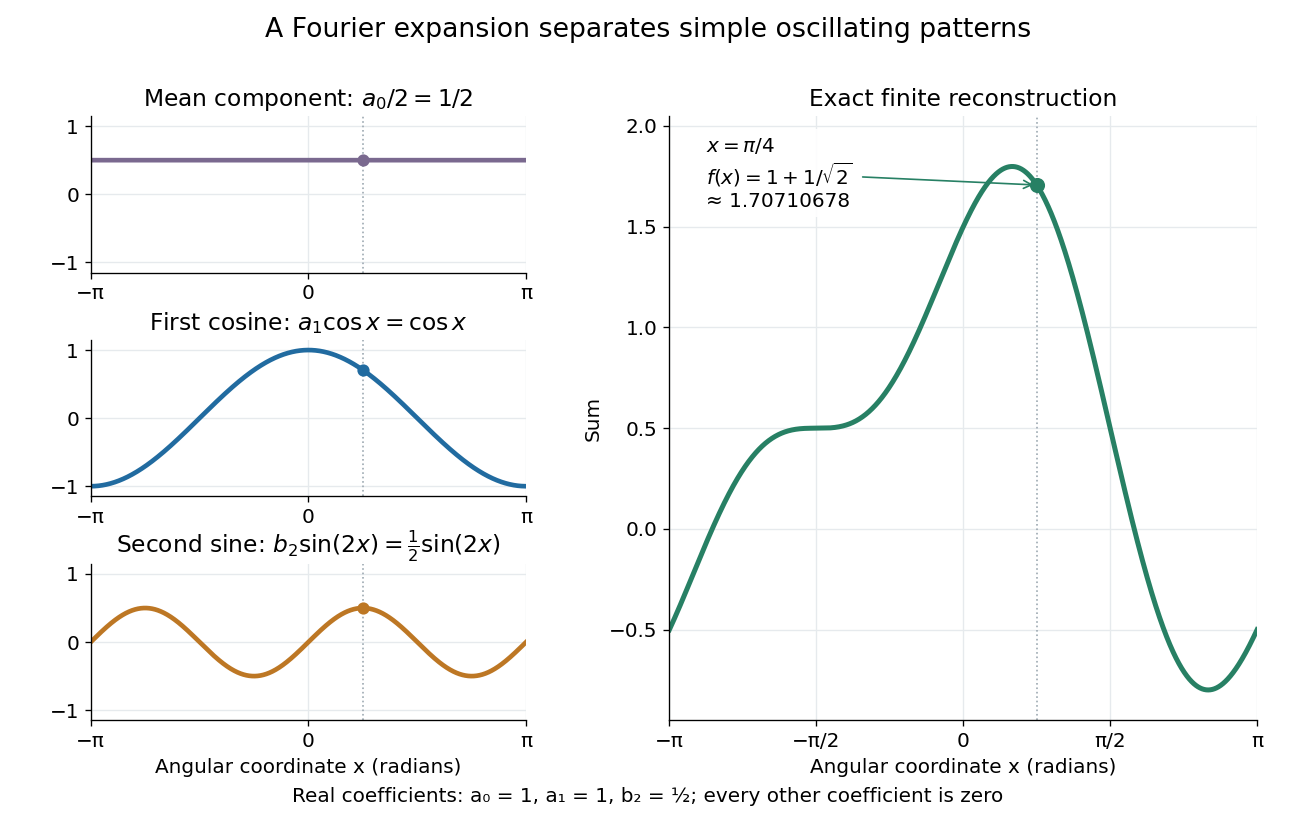
The change of viewpoint is useful because many linear problems act separately on these modes. The second derivative maps $\sin (nx)$ to $-n^2\sin (nx)$ and maps $\cos (nx)$ in the same way. Consequently a differential equation that is complicated for a whole profile can become a simpler calculation for each Fourier harmonic. A linear time-invariant system similarly has a separate response to each complex exponential. Superposition combines the responses when the relevant sums and operations are justified. ^[ref].

The infinite case contains a subtlety absent from the finite example. Under pointwise convergence of a piecewise smooth Fourier series, the value at a jump discontinuity is the average of the two one-sided limits. For a square-integrable function, the complex Fourier series instead converges in the $L^2$ norm: the integrated squared error tends to zero. Neither statement says that the error becomes small everywhere at once. A square wave shows the difference vividly through the Gibbs phenomenon.

A historical source for this connection between profiles and modes is Joseph Fourier's 1822 book Théorie analytique de la chaleur. Chapter III develops expansions in sines and cosines while studying the propagation of heat. The heat equation gives a continuing application of this approach. ^[ref].

First-step analysis conditions on the first transition of a stochastic process, turning hitting probabilities, hitting times, and accumulated rewards into linear recurrence equations.

A quantity $E(t)$ undergoes exponential decay with rate $\gamma >0$ when

For $I[y]={\int }_a^{b}F(x,y,y^{\prime })dx$, stationarity under fixed-endpoint variations gives

If $g(t,x)$ and its partial derivative $D_{i}g(t,x)$ are continuous for $t$ in a compact interval and $x$ in an open set, thenApply the fundamental theorem of calculus to the difference quotient in the $i$th coordinate and use uniform continuity on a compact neighbourhood.

For a smooth function $f:U\to \mathbb{R}$ on an open set $U\subseteq {\mathbb{R}}^n$, a critical point is an input $x_{\ast }$ where the gradient vanishes: $\nabla f(x_{\ast })=0$. Equivalently, every first partial derivative is zero. Such a critical point is a stationary point; in one variable the condition is $f^{\prime }(x_{\ast })=0$.

There is a broader convention in elementary one-variable calculus: a "critical number" is an interior input where the derivative is zero or does not exist, provided the function itself is defined there. Thus a corner can be a critical number without being a stationary point. Here the smooth meaning of critical point is used unless the broader convention is explicitly stated. ^[ref]

For the polynomial $f(x)=x^4-2x^2$ on the real line,The stationary points at $x=\pm 1$ are strict local minima and attain the global minimum; the stationary point at $x=0$ is a strict local maximum. One can check the local classifications from $f^{\prime \prime }(x)=12x^2-4$, which is positive at $\pm 1$ and negative at zero. The identity $f(x)=(x^2-1{)}^2-1\ge -1$ proves the global minimum directly. Since $f(x)\to +\infty$ as $|x|\to \infty$, there is no global maximum on $\mathbb{R}$.

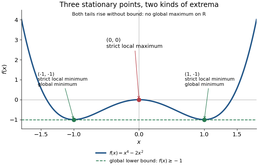
A zero derivative alone does not guarantee an extremum. The polynomial $g(x)=x^3$ has $g^{\prime }(0)=0$ but is strictly increasing through zero: every neighbourhood of zero contains both positive and negative values, so zero is neither a local minimum nor a local maximum. Conversely, the absolute value function $h(x)=|x|$ has a strict local minimum and a unique global minimum at zero, but its left and right derivatives are $-1$ and $+1$. It is not differentiable there, so zero is a critical number under the broader convention and is not a stationary point.

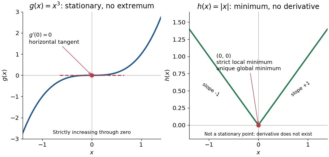
The usefulness of critical points is that they reduce the search for smooth interior extrema to equations. Every local minimum or local maximum of a differentiable function at an interior point has zero gradient; this condition is necessary, and $x^3$ shows that it is not sufficient. The striking feature is that all the first directional derivatives must vanish together, even though the surrounding values can form a valley, a peak, or a saddle point of a scalar function. ^[ref]

Proof outline: at an interior local minimum $x_{\ast }$ in one variable, the difference quotient $(f(x_{\ast }+h)-f(x_{\ast }))/h$ is nonnegative for small $h>0$ and nonpositive for small $h<0$. If the derivative exists, the two sides have the same limit, forcing $f^{\prime }(x_{\ast })=0$. Reverse the inequalities for a local maximum. In several variables, apply this argument along each coordinate line to obtain zero partial derivatives and hence zero gradient. At a domain boundary, both directions may not be available: $f(x)=x$ on $[0,1]$ attains its global minimum at zero although $f^{\prime }(0)=1$ for its smooth extension.

For $z=r{e}^{i\theta }\ne 0$, the complex logarithm has the values $\log r+i(\theta +2\pi k)$ for $k\in \mathbb{Z}$.