
For functions and , their function composition is , defined by . The rightmost function is applied first. Matching the intermediate codomain and domain of a function makes the expression well-defined.
For self-maps of the real numbers, take and . Then , whereas . Thus function composition need not be commutative. It does have the associative property: both and evaluate to whenever each intermediate codomain matches the next domain of a function. The identity function leaves composition unchanged, making self-maps particularly useful as a monoid of transformations.
A finite field is a field with finitely many elements: addition, subtraction, multiplication, and division by a nonzero element all stay inside a finite collection. Write , or , for a finite field with elements. The subscript counts elements; it does not prescribe modular arithmetic modulo . The field with four elements is the smallest example where that distinction matters.
Every finite field has size , where is a prime number and is a positive integer. To see the counting mechanism, use its prime field : the finite field is a finite-dimensional vector space over . For a basis , every element has exactly one expressionEach coefficient has choices, so there are expressions. Here is the characteristic of a field and is the dimension of a vector space. Thus sizes are possible, whereas are not prime powers and cannot be finite field sizes.
Conversely, every prime power occurs, and any two finite fields of the same size admit a field isomorphism. These are classification statements, beyond the counting argument. See Conrad's Theorems 1.5, 2.2, and 2.7.[ref]
https://kconrad.math.uconn.edu/blurbs/galoistheory/finitefields.pdf. Keith Conrad, Finite Fields, sections 1–2
Uniqueness means the arithmetic agrees after relabeling; it does not choose a basis, an irreducible polynomial for a quotient ring representation, or a particular field isomorphism. Even for the field with four elements, exchanging and preserves the arithmetic.The appeal for coding theory is exact, finite arithmetic with reliable division: polynomial interpolation and linear algebra work over a finite alphabet. A Reed-Solomon code represents messages by polynomials and adds redundancy by evaluating them at several distinct finite field elements. Forney's MIT notes develop this arithmetic as preparation for such error-correcting codes.[ref]
https://ocw.mit.edu/courses/6-451-principles-of-digital-communication-ii-spring-2005/8921c013c1d7802bb197572c52442b97_chap7.pdf. G. David Forney Jr., Introduction to finite fields, 2005
In cryptography, finite fields likewise supply exact arithmetic on finitely many symbols, with operations that can be implemented using bits.Historically, Évariste Galois published work on finite fields beyond prime fields in 1830, constructing them by adjoining elements satisfying irreducible polynomials over prime fields. Conrad's historical account also records E. H. Moore's 1893 terminology, from which the name Galois field and notation descend.[ref]
A countable set is a set that admits an injective function into the natural numbers. It is therefore either a finite set or a countably infinite set.
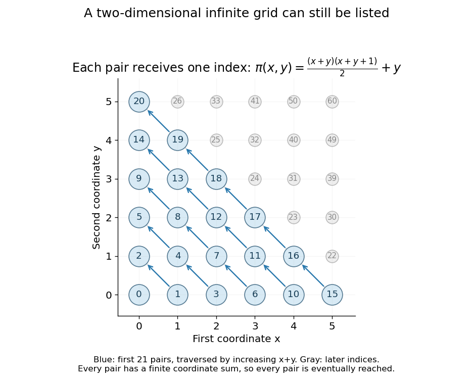
For a countably infinite set, countability means that its members can be arranged as a sequence in which every member occurs exactly once. The order need not resemble the order already present in the set. For example, the integers can be listed as . Simply increasing through positive values would never reach a negative one.
The Cartesian product needs a similar change of strategy. Listing a whole horizontal row first would never finish that row, so later rows would be missed. Instead list pairs by increasing coordinate sum , and within each finite diagonal by increasing :Every pair has a finite coordinate sum and therefore appears after finitely many earlier pairs. This is the construction made explicit by the Cantor pairing function. It explains why having two infinite coordinates does not, by itself, mean a larger cardinality.

A square root of an element is an element such that . The notation denotes the nonnegative square root when is a nonnegative real number.
Linear algebra studies vector spaces and linear maps: operations that preserve vector addition and scalar multiplication. For a linear map , the defining rule is , where are vectors and belong to the underlying field. The vectors might be arrows, lists of measurements, or polynomials. What matters is that their linear combinations make sense and that the same rule governs their transformation.
A concrete linear map is . Its two outputs record a sum and a difference. Since and , we immediately obtain . Knowing the outputs of the basis vectors determines the output of every vector; a matrix stores exactly that information in its columns.
The attraction of linear algebra is that one small collection of ideas answers several different questions. A system of linear equations asks which inputs produce a prescribed output. The image of a linear map describes the attainable outputs, while the kernel describes the invisible input changes. A basis gives every vector an address, and change of basis lets us choose addresses that make a linear map easier to understand. This shared language turns a collection of separate calculations into a picture of what is possible and how much freedom remains. Gilbert Strang's MIT course emphasizes these connections and their usefulness across other disciplines.[ref]
https://ocw.mit.edu/courses/18-06-linear-algebra-spring-2010/. Strang, MIT 18.06: Linear Algebra
Coding theory studies representations of messages that make decoding efficient, reliable, or compact. In channel coding, messages are mapped to separated codewords, so a corrupted word can still be recognized as coming from one particular message. In lossless source coding, a prefix code instead assigns short descriptions to frequent symbols. The objectives differ, but both exploit structure in the set of allowed words.
The simplest error-correction example sends as and as . If the receiver sees , at most one bit flip is consistent with , whereas two flips would be needed to obtain it from . A repetition code therefore recovers the original by taking the majority function of the received bits. The Hamming distance between the valid codewords is three: the spaces of one-error outputs around them do not overlap. This turns error correction into geometry in a discrete space.
The central tradeoff is between code rate and minimum distance. Additional separation makes correction possible but leaves fewer words available for messages at a fixed length. The Hamming bound counts disjoint error neighborhoods, while linear codes turn encoding and error detection into computations with matrices over finite fields. These connections explain why combinatorics, linear algebra, and probability theory all enter the subject.
Richard W. Hamming's Error Detecting and Error Correcting Codes appeared in the Bell System Technical Journal in April 1950, pp. 147–160. Its introduction motivates automatic correction through failures in digital computing, and its constructions go beyond detecting an error to identifying and correcting its location.[ref]
https://zoo.cs.yale.edu/classes/cs323/doc/Hamming.pdf. Hamming, Error Detecting and Error Correcting Codes, 1950
Representation theory describes abstract symmetries by linear maps on vector spaces. A group representation assigns an invertible linear map to each group element, respecting multiplication. The payoff is that a symmetry problem becomes a problem about matrices, invariant subspaces, and eigenvalues. Decomposing the action can reveal combinations of variables that a symmetric system cannot mix.
Take the cyclic group , with . On three real coordinates, let send to :This permutation representation does more than relabel a list: it acts linearly on every possible assignment of values to the three positions. The vector stays fixed. The vector subspace is also preserved, since a permutation does not change the sum.
Every vector separates uniquely into these two types:For example, . The first term belongs to a trivial representation; the second is a contrast with zero coordinate sum. This is a direct sum decomposition . The symmetry preserves the mean and rotates the contrasts.
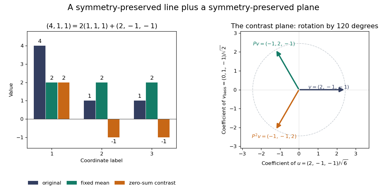
Three-coordinate cyclic symmetry preserves the mean and rotates the zero-sum contrasts by 120 degrees
. Details. 
The rotation is literal after choosing the orthonormal basis , of . In this basis,It is a rotation through degrees, and three applications return to the starting point. There is no nonzero invariant real line, because this rotation has no real eigenvector. Thus the two-dimensional action is an irreducible representation over the real numbers. Over the complex numbers it instead splits into two eigenlines with eigenvalues and . The coefficient field is part of an irreducibility claim.
Why would this decomposition matter for a physical calculation? Consider three equal masses with scalar displacements and the symmetric quadratic coupling energyThe equations of motion are , whereis a Graph Laplacian and is the all-ones matrix. The constant vector has eigenvalue zero: translating all coordinates equally costs no coupling energy. On , vanishes and , so both independent contrast directions have angular frequency . A three-coordinate coupled problem reduces to a free mean and two identical harmonic oscillators.
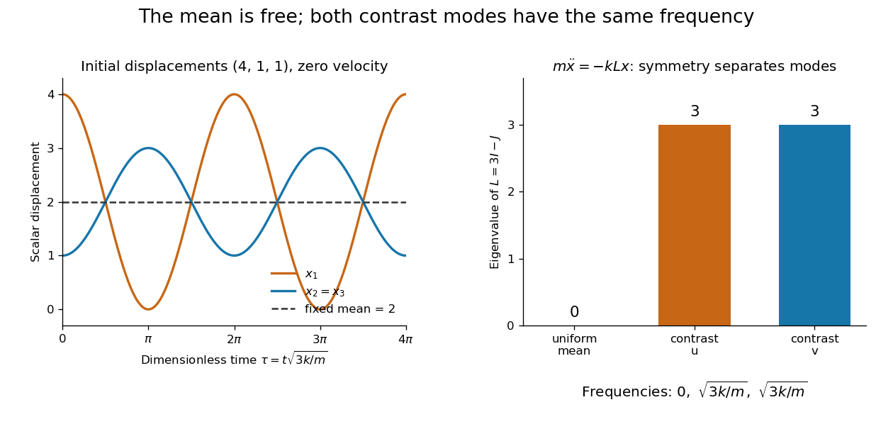
Equal pair couplings leave the mean fixed and make two independent zero-sum modes oscillate at the same frequency
. Details. 
For initial displacement and initial velocity zero, the exact solution is . The fixed mean and oscillating contrast can be read directly from the decomposition. More generally, a linear operator commuting with the group action carries its fixed-vector subspace into itself; with an invariant inner product, it preserves the corresponding orthogonal complement too.
For a finite group, averaging over the action constructs an invariant inner product over the real numbers or complex numbers. The resulting invariant complements explain Maschke's theorem: a finite-dimensional group representation decomposes into irreducible representations. Characters compress the action into traces and help identify those pieces. The assumptions matter; in modular representation theory the coefficient field can have characteristic dividing the group order, and such decompositions can fail. Chapter 4 of Pavel Etingof and coauthors' notes develops these mechanisms. [ref]
https://math.mit.edu/~etingof/reprbook.pdf. Etingof and coauthors: Introduction to representation theory
.Algebraic number theory studies integer factorization, divisibility, prime ideals, and units after extending the rational numbers to a number field. Its basic objects are a number field and its ring of integers : the counterparts of and . The field norm turns multiplication in into multiplication of rational numbers, and takes algebraic integers to integers. These connections let linear algebra and Euclidean geometry answer arithmetic questions.[ref]
https://www.jmilne.org/math/CourseNotes/ANT.pdf. J. S. Milne, Algebraic Number Theory, introduction and Chapter 2
A first example is with ring of integers . The integer acquires the factorizationEach factor has field norm . Neither is a unit, and each is an irreducible element: any factorization into two nonunits would factor the prime number into two integers of absolute value greater than one. Arithmetic in a larger ring thus reveals structure invisible in ordinary integer factorization.
There is also a complication: unique factorization of elements can fail, as in the failure of unique factorization in the ring of integers generated by square root of minus five. The general replacement is prime ideal factorization. The ideal class group measures the obstruction to making every ideal a principal ideal.
The historical motivation is visible in Richard Dedekind's original 1877 exposition: he begins with ordinary integer factorization, passes to Gaussian integers, and then uses a quadratic example to explain why ideals are needed. His later section establishes unique factorization of ideals in a number field. This is a direct record of the development of the theory, rather than a claim that all its ideas originated in one year.[ref]
https://www.numdam.org/item/BSMA_1877_2_1_1_69_0.pdf. Richard Dedekind, Sur la théorie des nombres entiers algébriques, 1877, Section II, §§5–10
[ref]https://www.numdam.org/item/BSMA_1877_2_1_1_207_1.pdf. Dedekind, continuation, 1877, §25
A polynomial is a finite sum of monomials with coefficients in a ring. In one variable over a commutative ring , writeThe symbol is an indeterminate: it records powers formally before we choose an input value. Finite expressions are easy to add, multiply, evaluate, and differentiate, making polynomials a common language for exact algebra and approximate numerical analysis.
Consider the real polynomialThe expanded form displays the coefficients and the degree of a polynomial; the factored form displays its roots of a polynomial. At , either description gives . At and , the factored form makes the zero values immediate. Keeping several descriptions of one object is useful because each makes a different question easy.
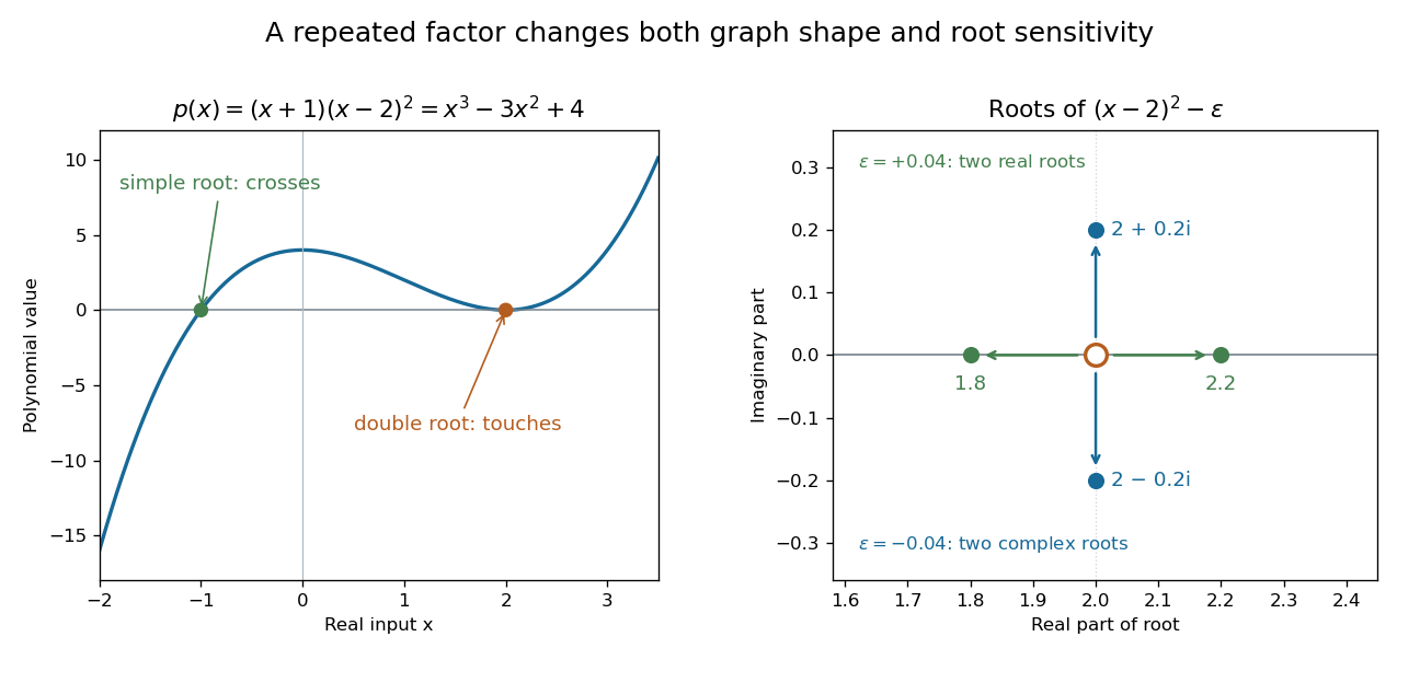
A simple polynomial root crosses the axis, while a double root touches it; perturbing the double factor can produce real or complex roots
. Details. 
The graph shows another connection. The factor changes sign across , while stays nonnegative across . Thus the graph crosses the axis at the simple root of a polynomial and touches it at the double root. Multiplicity of a root turns an algebraic repetition into visible local behavior.
For calculations, Horner's method evaluates a polynomial through nested multiplication. For modeling, a Taylor polynomial describes local behavior near a point, while polynomial interpolation constructs a polynomial matching prescribed data. Their usefulness comes with assumptions: a local approximation and an exact identity are different claims, and changing the coefficient ring can change which polynomial roots exist.
A field is a commutative ring with in which every nonzero element has a multiplicative inverse. Examples include the rational numbers, real numbers, and complex numbers. The integers are a ring but not a field: dividing by leaves them. For a prime number , the prime field is a finite example, because every nonzero residue is coprime to and hence has a modular inverse.
In , the nonzero inverse pairs are , , , and . Thus has solution in this field; the real number solution would be . Dividing by a nonzero coefficient is valid in both settings, but it means division according to the chosen field's operations.
A field has no zero divisors: if and , multiplying by gives . This short argument supports polynomial factorization arguments and pivot division in Gaussian elimination. It does not hold in every commutative ring: modulo , the nonzero residues and multiply to zero. The distinction is visible in the figure under algebraic structure.
A sphere of volume translating through unbounded inviscid incompressible fluid has fluid kinetic energyIts added mass is therefore one half of the displaced fluid mass.
There are unlisted articles, also show them or only show them.