
An asymptotic expansion describes a function near a specified limit by successively smaller scales. Each fixed finite truncation has a remainder smaller than its last retained scale. The central question is how the approximation improves as the parameter approaches the limit; convergence of the entire infinite series at a fixed parameter is a separate question. For the inverse-power scale ,means that, for every fixed nonnegative integer ,The little o notation makes the accuracy requirement precise. With expansions to all orders, this is also equivalent to an remainder after the th term; the implied bound may depend on .[ref]
For a quick convergent example, the finite geometric series identity givesFor , both the asymptotic expansion as and the ordinary convergent geometric series describe this function. The exact remainder displays the required extra inverse power.
The more surprising example under a divergent factorial series can approximate a convergent integral has a convergent integral but a divergent series at every fixed positive :A few terms can estimate well, even though adding sufficiently many terms eventually destroys the approximation. Optimal truncation explains where to stop.
This makes asymptotic expansions useful when an exact expression is a complicated integral or differential equation solution, but a parameter is very large or very small. The leading term reveals the scale; corrections reveal which effects matter next. The asymptotic sequence must be specified: integer powers, fractional powers, logarithms, and exponential functions can encode different kinds of behavior. A good finite approximation includes a remainder estimate or an independently checked range of use.
Numerical analysis designs algorithms that approximate mathematical answers while controlling cost and error. Its central question is how much of a computed answer can be trusted. Finding a zero of a function, evaluating an integral, solving a linear system, and evolving an ordinary differential equation all demand choices about accuracy, work, and the information available. MIT's numerical-methods course explicitly treats performance and accuracy as joint concerns.[ref]
https://ocw.mit.edu/courses/18-335j-introduction-to-numerical-methods-spring-2019/pages/week-1/. Steven G. Johnson, MIT 18.335J, Week 1, 2019
Three questions organize error analysis. Truncation error measures the approximation introduced by an algorithm even in exact arithmetic; roundoff error comes from finite precision; the condition number measures sensitivity inherent in the problem. Numerical stability asks how the chosen algorithm propagates perturbations. These distinctions suggest different remedies: refine an approximation, change precision or arithmetic, or improve the accuracy of the input.
For example, the square root has relative condition number for : a small relative change in produces about half that relative change in . In contrast, has relative condition number . Changing to changes to about : an input change of about produces an output change of about . This sensitivity exists even with exact arithmetic. MIT's conditioning lecture separates the condition number from roundoff error in precisely this way.[ref]
https://ocw.mit.edu/courses/18-335j-introduction-to-numerical-methods-spring-2019/pages/week-2/. Steven G. Johnson, MIT 18.335J, Lecture 5: Condition Numbers, 2019
Oscillatory integrals are led by points where the phase derivative vanishes, with a phase shift determined by the Hessian signature.
The upper incomplete gamma function is under the convention used here.
The unilateral Laplace transform of a function is the integral transformHere is a complex number, is its real part, and is the imaginary unit. The exponential function factor weights the history, while probes its oscillations. The integral starts at zero, so it uses only the history from that starting time onward. This section concerns ordinary functions; their value at the single endpoint does not change the integral. See MIT 18.03SC, definition and elementary examples.
The Laplace transform is useful because it packages an entire time history into a function of : a derivative becomes multiplication by together with the initial value, and a convolution becomes a product. Thus a linear differential equation can become an algebraic equation that already remembers its initial value problem. The worked example below shows both descriptions of the same response.
If is a piecewise continuous function and has exponential order , then its defining integral is absolutely convergent for . This is a sufficient condition; the actual Laplace convergence region may be larger than the bound obtained from a chosen . [ref]
https://ocw.mit.edu/courses/18-03sc-differential-equations-fall-2011/fff4420903d82c5c5c483e54566bc5ec_MIT18_03SCF11_s27_2text.pdf. MIT 18.03SC, domain and growth conditions
.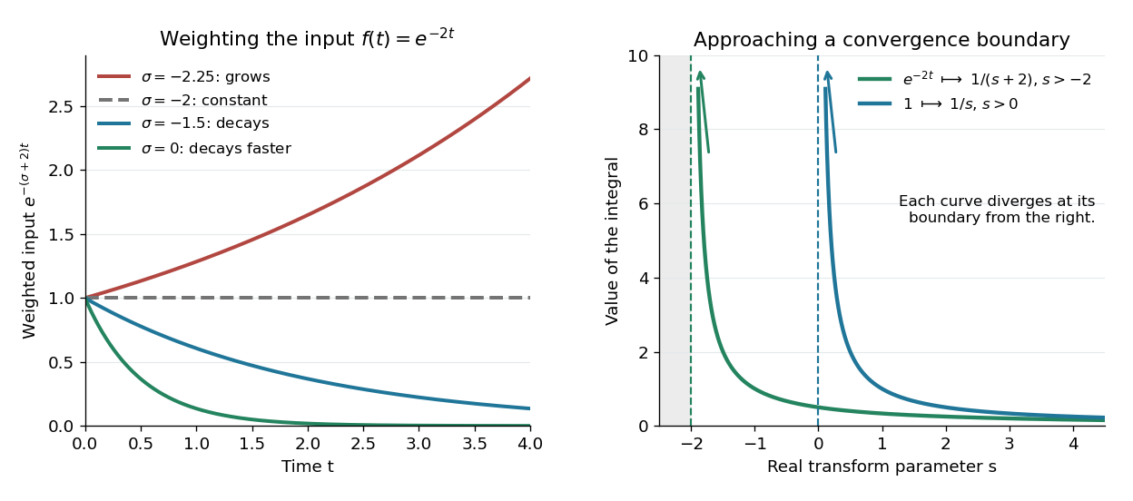
The bound has a short explanation. For sufficiently large , , so , whose tail integral is finite for . The finite initial interval is covered by piecewise continuity.
Three calculations make the convergence condition concrete. For the input , evaluate the finite-history integral first:At the finite-history integral is . For the exponential function input , the same calculation replaces by , givingIn particular, is allowed for this decaying input: its weighted integral is . For the sine input, Euler's formula gives ; linearity then yieldsThe Laplace convergence region is part of the answer. For example, has an analytic continuation to , but the defining integral for the input diverges there. The sine calculation is also developed in MIT 18.03SC, further elementary transforms.
To see why the initial value appears, suppose is an absolutely continuous function on every finite interval , with its right one-sided limit. At the chosen , assume and are Lebesgue integrable functions and . The Laplace transform of a derivative is thenFor example, exponential order bounds on both and guarantee these conditions whenever exceeds both growth bounds. The initial value is the lower-end boundary contribution of integration by parts.
Consider the initial value problemWrite . The Laplace transform of a derivative and linearity give for . A partial fraction decomposition therefore givesWe recognize the two elementary Laplace transforms already computed. Directly verify the result: its derivative is , soThis verifies both the ordinary differential equation and the initial value, and shows that the resulting bounded function has the Laplace transform used above. The response rises from zero toward : at that value the input balances the term . The general method is described in MIT 18.03SC, solving initial value problems.
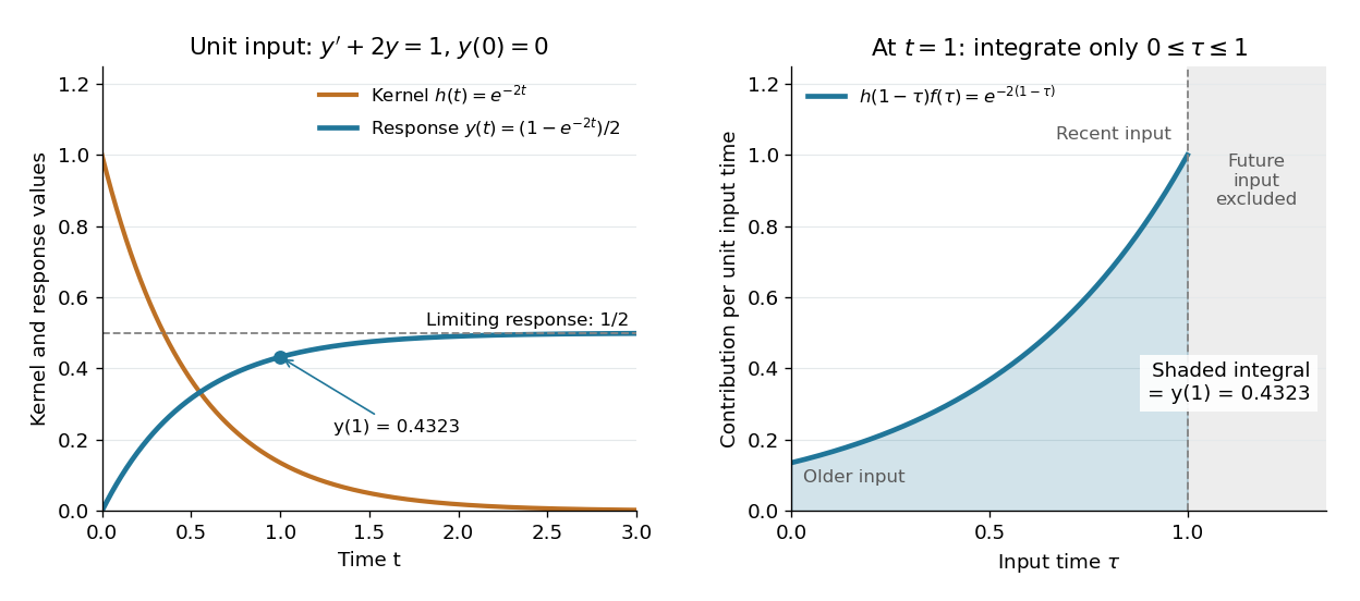
The same solution is a convolution. For functions defined on , the unilateral convolution isThe main convolution article integrates over the whole real line; applying a causal extension by zero to both functions makes its formula identical to this one. Nonzero contributions require both and , hence . If and are Lebesgue integrable functions on , the convolution theorem for Laplace transforms statesFor piecewise continuous functions of exponential order and , it holds throughout . The weighted absolute double integral factors into the two finite weighted absolute integrals; Fubini's theorem therefore permits exchanging the order, and setting separates the product. [ref]
https://ocw.mit.edu/courses/18-03sc-differential-equations-fall-2011/0d4d90053f2bb24f7551c78e2d1b21a2_MIT18_03SCF11_s30_5text.pdf. MIT 18.03SC, convolution and system response
.For the linear time-invariant system starting at zero, the convolution kernel is its impulse response for , extended by zero for . With the Heaviside step function input, for , the accumulated response isThus on is both the algebraic solution and the Laplace transform of a finite-history convolution. Each past input contributes an exponential function that decays with its age , which makes the two descriptions easy to connect.
Finally, compare the Fourier transform convention . If is the causal extension by zero of , define . Whenever is a Lebesgue integrable function,A vertical slice of the Laplace transform is therefore the Fourier transform of the zero-extended, weighted input. Positive damps its positive-time history. A finite window function instead gives and ; this approaches in the Laplace convergence region. Setting directly requires an integrable zero-extended input: the input fails that condition, even though its Laplace transform exists for every .
The history of the Laplace transform spans several stages. Schiff's historical summary notes that Laplace's 1812 treatise acknowledged earlier work on integral transforms and describes later development of the modern Laplace transform method. [ref]
https://oldversion.stu.edu.vn/uploads/documents/170509-091205.pdf#page=9. Schiff, The Laplace Transform: Theory and Applications, historical summary, pp. x–xi
.Complex analysis studies functions of a complex number, especially holomorphic functions. Its distinctive feature is that a single complex derivative controls variation in every direction of the complex plane. The map gives a first picture: straight coordinate lines become curved, yet small perpendicular arrows remain perpendicular wherever .
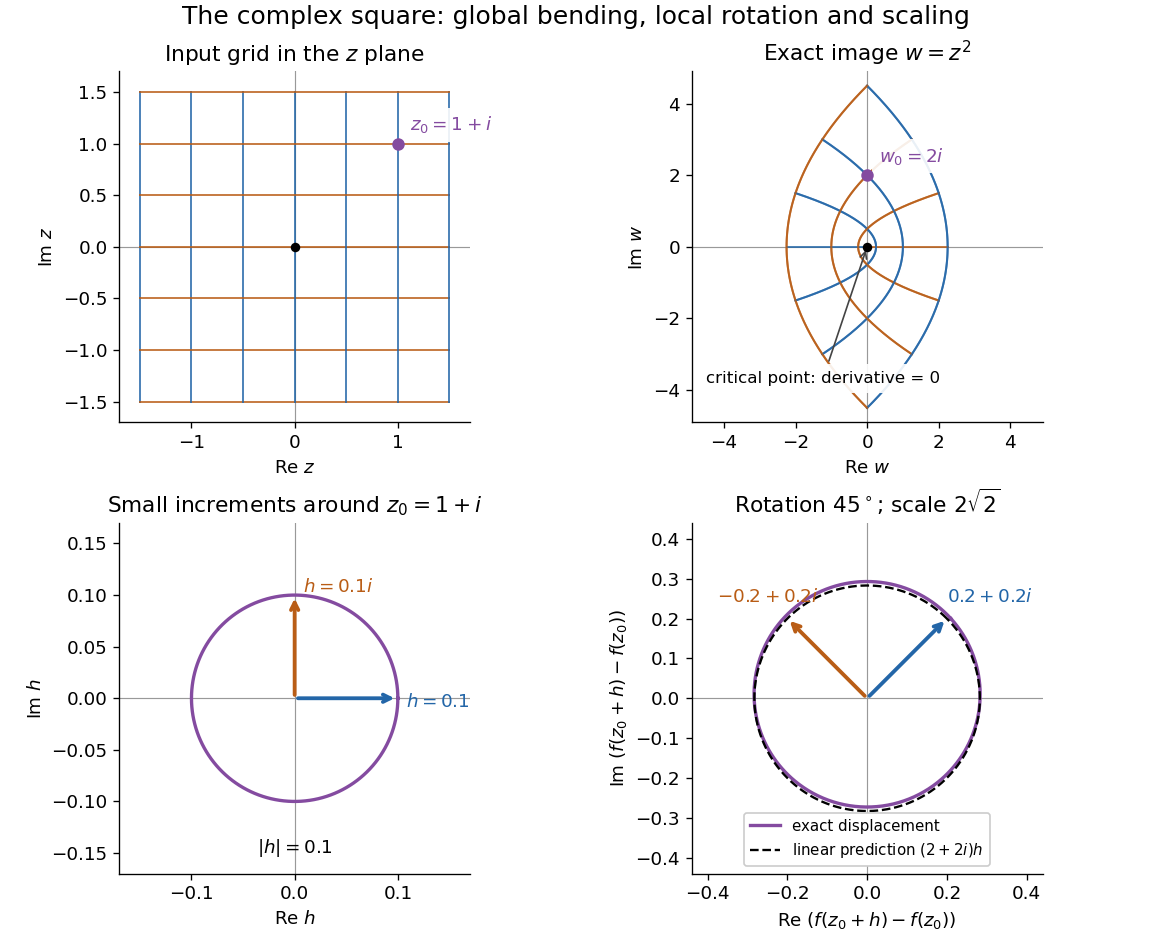
The complex square bends a grid globally and acts near 1 + i as a rotation through 45 degrees and a scaling by twice the square root of two
. Details. The bottom panels show displacements rather than absolute positions. Multiplication by predicts the image of each small arrow; the exact image differs by . The origin is exceptional because . This distinction between local conformal maps and a critical point is central: complex differentiability imposes strong geometric structure, without making every holomorphic function globally one-to-one.
The remarkable next step is that holomorphic functions are determined inside a circle by their values on its boundary. Precisely, let , let , and suppose is a holomorphic function on an open set containing the closed disc . Orient its boundary counterclockwise. The Cauchy integral formula states that, for every ,The contour integral combines boundary values with a kernel depending on the requested interior point. It is a reconstruction formula, not merely a trick for evaluating an integral. The hypothesis about the closed disc ensures that all boundary values and the contour integral are well defined. [ref]
At the centre, substituting cancels the denominator against :Thus the centre value is the angular average of the boundary values. For the polynomial , and , expand the boundary data asBoth oscillating terms have zero average, leaving . Away from the centre the weights change: on the unit circle,With and , expanding the denominator as a geometric series leaves only its second-power term after integration, giving . This also explains how the Cauchy integral formula recovers an entire Taylor series from boundary data.
When a holomorphic function has isolated singularities, a different boundary calculation detects their residues. Suppose is a counterclockwise simple closed contour and is holomorphic on a neighbourhood of it and its interior except at finitely many interior isolated singularities . The residue theorem givesA residue is the coefficient of in the Laurent series. A short proof idea is to deform the contour to small circles around the isolated singularities using the Cauchy integral theorem. Integrating the Laurent series on each circle kills every power except . [ref]
Here is how a complex pole determines a real improper integral. Set and use the contour consisting of the segment from to , followed by the upper semicircle , with . Only the simple pole lies inside, andThe arc must actually disappear. On , the reverse triangle inequality gives , and its length is , soThe real integrand is bounded by for , so both tails converge separately. Taking the limit therefore proves the ordinary improper integralFor example, at the real segment contributes , and the arc contributes , below the bound . The usefulness of the residue theorem is that the same strategy works for many rational functions whose real antiderivatives are cumbersome: find the enclosed poles, compute their residues, and control the connecting arc. [ref]
https://ocw.mit.edu/courses/18-04-complex-variables-with-applications-spring-2018/f69bc227ae476839819fb18e5b283072_MIT18_04S18_topic9.pdf. Orloff, MIT Topic 9, contour decay estimates
Historically, Cauchy's 1825 memoir on integrals with imaginary limits develops complex contour integration and its use in transforming and evaluating definite integrals. The opening sections define complex path integrals, discuss changing the path, and examine what happens near singular points. These are recognizable ancestors of the modern link between holomorphic functions, contours and residues. [ref]
https://www.numdam.org/item/BSMA_1874__7__265_0.pdf. Cauchy, Mémoire sur les intégrales définies, prises entre des limites imaginaires, 1825; reprinted 1874, sections 1–6
Fourier analysis describes a function by the oscillations that compose it. A graph records values at successive positions or times; a frequency spectrum records how much of each frequency is present, together with its wave phase. The same complicated shape can become a short list of simple components. For periodic functions, the components form a Fourier series; on the whole real line, the Fourier transform uses a continuous range of frequencies, and the Fourier inversion theorem puts them back together.
For a concrete example, consider the trigonometric polynomialWith measured in seconds, its three Fourier harmonics have frequencies , , and cycles per second and amplitudes , , and . Each cosine has zero wave phase. Adding them creates the sharper peaks in the figure. The frequency spectrum makes the recipe immediately visible; changing an amplitude changes the shape without changing the component's frequency. Fourier orthogonality lets us recover each Fourier coefficient by averaging against the corresponding sine or cosine, because the other Fourier harmonics cancel over a full period of a function.
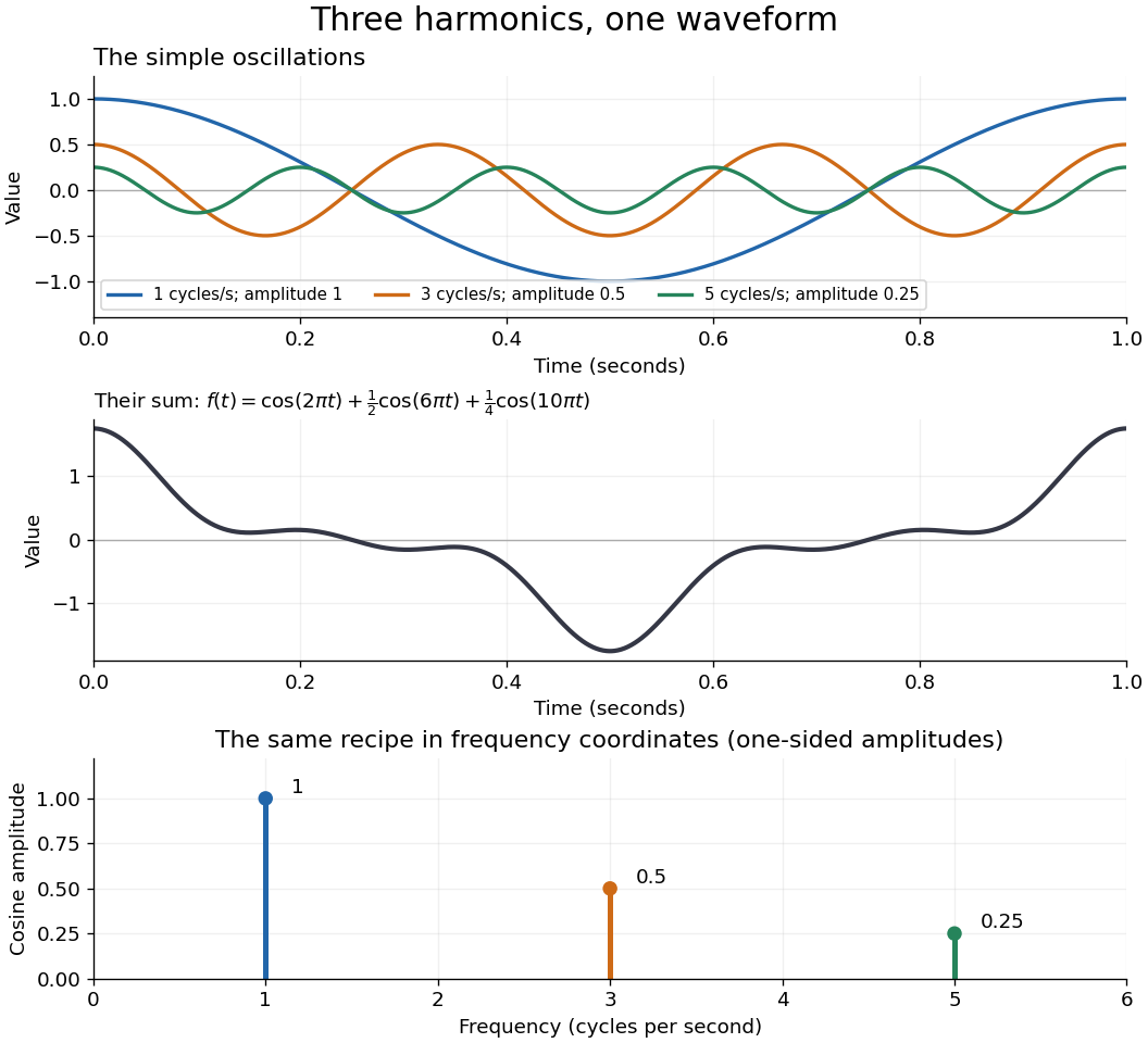


The deeper reason these components are so useful is that they simplify operations. By Euler's formula, the exponential function packages a cosine and a sine into one Fourier mode. A translation or a derivative changes only its multiplier:Thus Fourier modes are simultaneous eigenfunctions of these operations. In Fourier series, this gives a literal diagonalization in the Fourier basis; on the real line, the Fourier transform gives the continuous counterpart, with each frequency handled separately. The Translation property of the Fourier transform and the Fourier transform of a derivative turn shifting and differentiating a whole function into multiplication of its Fourier transform. A convolution likewise becomes multiplication by the convolution theorem. This is beautiful because one description simplifies several apparently different operations at once.
For example, the heat equation , with thermal diffusivity , evolves a spatial Fourier mode asFine ripples have larger angular frequencies and decay faster: the formula explains why heating smooths a jagged temperature profile. For a general initial profile with sufficient regularity, the Fourier transform gives , and Fourier inversion recovers the temperature. Similarly, multiplying selected parts of a frequency spectrum suppresses unwanted components. Claude E. Shannon's Communication in the Presence of Noise (1949), Section III, describes ideal filtering as a projection that retains some frequency coordinates and removes others.[ref]
https://fab.cba.mit.edu/classes/S62.12/docs/Shannon_noise.pdf. Shannon 1949, Section III, p. 13: filtering in frequency coordinates
The physical motivation is already visible in Joseph Fourier's Théorie analytique de la chaleur (1822). Chapter III constructs heat profiles using sums of sines and cosines; Chapter IX, articles 355–359, passes from Fourier series to integrals as the spatial interval becomes unbounded. These heat problems explain the motivation for the discrete and continuous descriptions. Their modern formulations specify which functions admit reconstruction and in what sense the expansions converge.[ref]
https://fr.wikisource.org/wiki/Th%C3%A9orie_analytique_de_la_chaleur/Chapitre_3. Fourier 1822, Chapter III: trigonometric representations of heat profiles
[ref]https://fr.wikisource.org/wiki/Th%C3%A9orie_analytique_de_la_chaleur/Chapitre_9. Fourier 1822, Chapter IX, articles 355–359: from series to integrals
Functional analysis brings linear algebra and topology together to study vector spaces of functions and the linear operators acting on them. A function space such as has infinitely many independent directions: the monomials are linearly independent. Finite linear combinations alone cannot describe all its continuous functions. A useful theory must also say when approximations converge, whether their limits belong to the chosen space, and which operations preserve that norm convergence. Normed vector spaces, Banach spaces, and bounded linear operators provide these three controls.[ref]
A bounded linear operator between normed vector spaces satisfies for every , with one finite constant . The least possible constant is its operator norm. By linearity, the same estimate controls approximation errors:This is exactly continuity for a linear map between normed vector spaces; neither space needs to be complete. It turns an input accuracy guarantee into an output accuracy guarantee, even when the input has infinitely many degrees of freedom.[ref]
https://ocw.mit.edu/courses/18-102-introduction-to-functional-analysis-spring-2021/22bf2f774fb161776032491568148707_MIT18_102s21_lec2.pdf. MIT 18.102, lecture 2: boundedness, continuity, and the operator norm
For a concrete linear functional on , take the integral . In the supremum norm,The constant function attains equality, so . For , the output is ; any approximation with therefore has . The Cauchy-Schwarz inequality also gives on this interval, again with equality at . Thus integration remains a bounded linear functional under the L2 norm, although point evaluation behaves very differently.
The beauty of this viewpoint is that one estimate can justify an entire approximation procedure. Once a sequence converges in the chosen norm, every bounded linear operator carries its limit along. Completeness ensures that Cauchy approximations actually describe an element of the space. The choice of norm matters: it determines which errors are small and which measurements are stable. The examples below distinguish an average, which ignores sufficiently narrow peaks, from point evaluation, which detects their full height. For applications, this decides whether reducing an overall fitting error guarantees an accurate reported measurement. A small L2 norm of the error controls its integral on this interval, while it gives no such guarantee for a single sampled value.
Nonlinear analysis studies equations and variational problems in which superposition fails. Its tools include nonlinear functional inequalities, conserved energies, compactness, phase-plane methods, and concentration arguments.
A power law is a relation , with fixed constants and . For positive , any real number is allowed. Its useful feature is a simple scaling rule:The same proportional change of input produces the same proportional change of output, independently of the starting value. The exponent controls that response; the coefficient fixes the magnitude.
For example, the area of a circle is . Doubling the radius multiplies its area by four, and tripling it multiplies the area by nine. The volume of a sphere is : the same changes multiply its volume by eight and twenty-seven. The distinction explains why similarly shaped objects do not preserve their ratio of surface area to volume when their size changes.
When the output is positive, a logarithm turns the power law into a straight-line relation. Using positive reference values and ,These ratios are dimensionless quantities, so the formula also applies to physical measurements with units. Plotting both ratios on a logarithmic scale gives a line of slope . Changing a unit changes the numerical coefficient, while the exponent stays the same. Positive describes increasing values; negative describes decreasing values; gives a constant. The zero coefficient is a degenerate case with no useful logarithmic slope.
Exact scaling is stronger than regular variation. The function has a doubling ratio tending to four, but its logarithmic correction keeps growing. The diagram contrasts it with the exact power law .
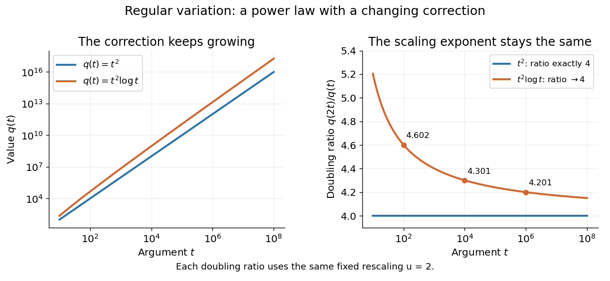
Exact quadratic scaling and a logarithmic correction have different finite doubling ratios, even though the correction leaves the limiting exponent unchanged
. Details. 
A power law for a probability density and a power law for a tail probability have different exponents. For a Pareto distribution with and lower endpoint one,The tail probability has exponent ; differentiating it and changing sign gives the probability density exponent . Confusing them changes the interpretation of a fitted exponent. The normalizing coefficient and lower endpoint also matter: a decreasing power law is not automatically a valid probability density over the entire positive real line.
The appearance of a line over a finite logarithmic range is evidence to investigate, rather than a proof of an exact power law or its mechanism. In their study of power-law distributions, Clauset, Shalizi and Newman combine maximum likelihood estimation, goodness-of-fit tests and comparisons with alternative models; their abstract explains why ordinary least-squares fitting can give misleading results for tail data. See Aaron Clauset, Cosma Rohilla Shalizi and M. E. J. Newman, Power-law distributions in empirical data, SIAM Review 51 (2009), 661–703. The scaling rule is mathematically exact when it defines a model; whether a dataset supports that model is a question of statistical inference.
Noncommutative algebra studies rings whose multiplication need not commute and their one-sided ideals and modules.
Commutative algebra studies commutative rings, ideals, modules, and the spectrum of a ring. Its basic question is which familiar rules of integer and polynomial arithmetic survive in a new setting. The distinction between units, zero divisors, and integral domains makes that question concrete.
There are unlisted articles, also show them or only show them.