
For a Lenard-Magri recursion, antisymmetry shifts an index: when . Repeating reaches , because is a Casimir function. The recursion then gives . This proof applies to every finite initial portion for the indices that can be shifted inside it, and to all pairs in an infinite sequence.
The next step of a Lenard-Magri recursion requires to be a Hamiltonian vector field for . It must be tangent to the symplectic leaves, and its contraction with the leaf symplectic form must have a global potential, with a compatible smooth extension between leaves. Even the first step may fail: on , take , and . Both Poisson structures are compatible, but cannot hold, because its left side is zero and its right side is nonzero.
With , the generating function satisfies . Expanding in Legendre polynomials gives . Boundedness at zero removes , and the value at makes . Orthogonality then gives . The integral is , so . Uniform analyticity on compact subdiscs justifies the generating expansion and termwise calculations.
Differentiating the Legendre differential equation gives for . Multiply the equations for two distinct indices by the opposite polynomial and subtract. The endpoint term vanishes because of , giving the displayed weighted orthogonality. The zero polynomial is not a nonzero eigenfunction.
For the centered two-level advection recurrence, the Fourier roots at Courant number one coalesce at for phase . The resulting nontrivial Jordan block admits linearly growing solutions despite both eigenvalues having modulus one. Uniform two-level stability for arbitrary starting perturbations therefore requires the strict inequality . A specially consistent startup can select the exact translating branch at the boundary, which is a restriction on the data rather than a uniform bound on the full update.
For with equal spatial mesh sizes, the centered leapfrog recurrence has amplification polynomial of a multilevel finite difference scheme . Uniform stability for arbitrary two-level starting perturbations holds exactly for . At the phase pair gives , and its companion matrix has a nontrivial Jordan block, producing growth proportional to the number of steps. For larger one polynomial root has modulus greater than one. Bounds on eigenvalue moduli alone therefore give a misleading non-strict endpoint.
A proper lattice ideal is prime if implies or . Its complement is a prime filter of a distributive lattice when the lattice is distributive: downward closure of the ideal makes the complement upward closed, primeness makes it meet-closed, and join closure makes that filter prime. Equivalently, its complement indicator is a homomorphism of lattices to the two-element lattice. Given in a distributive lattice, maximize an ideal containing and avoiding using Zorn lemma. If lie outside it, the two enlarged ideals contain , so and for some . Distributivity shows that would force , a contradiction. Thus this maximal avoiding ideal is prime and separates the two specified elements.
The Laplace radius is the satellite distance where the small-tilt nodal precession contributions from a planet's axisymmetric quadrupole and the stellar tide have equal magnitudes. In the circular hierarchical limit those rates are and . Equating them proves the displayed fifth-root expression. Inside this radius the planetary quadrupole coefficient controls the preferred plane; outside it the double-averaged circular tidal potential dominates. When equator and planetary orbit are inclined to one another, their balance determines the local Laplace plane.
For the Lang map, . This twisted right-translation identity determines which subgroups act on its inverse images. Fibres are left -cosets, by the Lang theorem for algebraic groups.
The signed third-order longitudinal structure function has this leading inertial range form under homogeneity, isotropy and the usual local-equilibrium scale separation. Its coefficient follows from the Kármán-Howarth equation and the mean kinetic energy budget, without assuming the Kolmogorov two-thirds law. Its negative sign encodes a forward energy cascade; it does not establish every higher-order similarity exponent.
A Kirby diagram depicts a handle decomposition of a four-dimensional manifold using a framed link for the two-handles and dotted circles for the one-handles. The framing specifies the attaching normal directions; it controls the resulting intersection form and the boundary Dehn surgery.
For an m-component integral framed surgery link, normalize its full colored bracket by the displayed expression, where is the signature of its linking matrix. The Kirby color handle-slide identity handles slides; cancels disjoint plus- or minus-one-framed unknots. Kirby calculus therefore makes this an oriented 3-manifold invariant. This convention has .
// Target: module-theory.bigb
The Fubini-Study metric is the standard unitary-invariant Kähler metric on Complex projective space, induced from the unit sphere by the Hopf fibration. Its associated Kähler form is the Fubini-Study form; scaling conventions determine the area of a projective line.
A predictable mark-dependent integrand gives a true martingale whenever on every finite horizon. Local versions follow when this expected integrability holds after localization. The compensator identity applied to predictable indicators from the past proves that every increment has conditional expectation zero. Choosing gives the generator martingale under the same local integrability conditions.
The predictable random measure matching the expected integrals of the jump measure against every nonnegative predictable integrand. For displacement marks of a Markov jump process, . Multiplying the integrand by an event known before an interval proves that the compensated integral has conditionally centered increments; expected absolute integrability makes it a true martingale. Squared-integrand integrability gives the square-integrable compensation isometry.
An electrical calorimetry experiment asks whether a measured electrical work input accounts for a measured warming. The University of Iowa's demonstration uses an insulated flask containing water, an immersed heater, a thermometer, electrical meters and a timer. Its procedure compares the duration, electrical readings and temperature rise. The following low-power measurement design and synthetic readout develop that idea; they are not measurements reported by the demonstration. [ref]
5F15.10 - Electrical Equivalent of Heat by University of Iowa Department of Physics and Astronomy. Equipment and Procedure: insulated flask, immersed heater, thermometry, electrical meters and timed warming
Use a covered calorimeter with weighed water, an immersed resistor, a calibrated thermometer and gentle stirring. Put an ammeter in series with the heater branch and a high-input-electrical resistance voltmeter across the immersed resistor's terminals. Record , , temperature and room temperature before, during and after switching the heater on. Measure the electric potential difference at the heater, rather than at the supply: lead and contact electrical resistance outside the receiving boundary can consume power that never reaches the water. Account for voltmeter loading if the ammeter also includes the sensing branch's electric current.[ref]
The electrical readout gives operating electrical resistance when , and power . To test Ohm's law, obtain several pairs at the same temperature; one ratio alone cannot establish a linear response. For small electrical resistance, use four-terminal sensing to exclude lead drops and reverse electric current to test stable offsets from the thermoelectric effect. Use brief low-power resistance measurements if the intended result is the unheated value: the test itself causes Joule heating.
For a covered assembly at approximately constant pressure, with negligible evaporation, negligible endpoint mechanical energy changes and no phase transition, takeHere is the water's specific heat capacity at constant pressure, is the participating vessel, heater and sensor heat capacity, is signed outward heat leakage, and is stirring work entering the assembly. The storage term approximates its enthalpy change; for a rigid fixed-volume receiver use the corresponding heat capacity at constant volume. Calibrate independently if the purpose is to test electrical input against thermal storage. Using the same heating run to define and then claiming it verifies the equality would be circular.
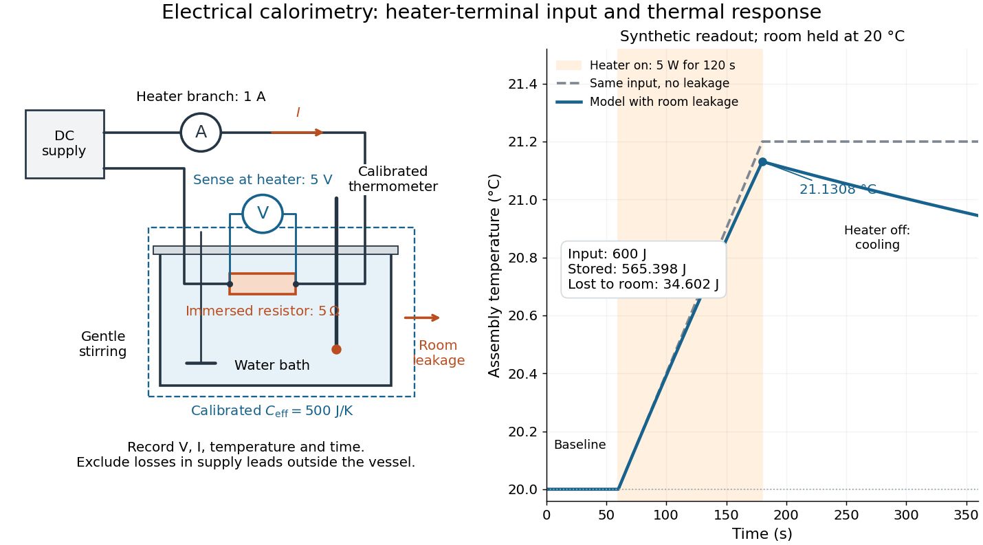

For the synthetic trace, stipulate , , , , room temperature , and loss coefficient , with negligible stirring input. The heater runs for , beginning at room temperature. The calorimeter heat-loss correction model isIt predicts , , storage and outward loss . Neglecting leakage undercounts deposited energy by about ; assuming no loss predicts . After switching off, the excess temperature undergoes exponential decay with time constant . A cooling slope can estimate only with known and a credible single-temperature model.
Controls separate causes of a temperature rise. Check the electrical meters' zeros and thermometer calibration; keep water mass, immersion, lid and stirring fixed between runs. Record a heater-off stirred baseline to estimate sensor drift and stirring input. Repeat cooling runs over the same temperature range to estimate environmental heat transfer; a baseline taken only at room temperature cannot measure warming-dependent leakage. Vary electric current while keeping and initial thermal conditions comparable: corrected deposited energy should scale as for equal durations. An independent calorimeter calibration or known reference heat capacity makes this a quantitative test rather than a qualitative observation.
Finite sensor response, incomplete thermal equilibrium, changing or heat capacity, evaporation, and imperfect loss corrections limit the inference. A final temperature alone cannot distinguish smaller electrical input from larger heat leakage or a larger participating heat capacity. Agreement tests the stated assembly and its energy accounting; it does not show that all electrical work in arbitrary devices becomes heat.
Historically, the Royal Society's archive description of James Prescott Joule's manuscript dated 13 October 1840 records a coil of wire in a jar of water, a thermometer and a galvanometer, and summarizes his inference that warming depends on electrical resistance and the square of electric current intensity. This electrical experiment precedes Joule's paddle-wheel experiment; the input here is electrical work, whereas the paddle supplies mechanical work. The catalogue, rather than the inaccessible manuscript images, supports this account. [ref]
Archive catalogue record AP-23-34: On the production of heat by voltaic electricity by The Royal Society Archives. Royal Society Archives, AP/23/34, Description and Date: apparatus, resistance dependence and duplicate-ratio conclusion; manuscript dated 13 October 1840
The electric field does work on matter at local power per volumeHere is current density and the dot product includes the relative direction. Positive means energy passes from the field to matter; negative means matter supplies energy to the field. In general this is a work rate, not automatically an irreversible heating rate.[ref]
For a stationary isotropic Ohmic conductor with real scalar electrical conductivity , local Ohm's law gives . Thus the local Joule heating rate isThe electrical resistivity has units , and electrical conductivity has units . These formulas use the material's rest frame and dissipative conduction current density. Moving media, complex conductivity, and additional storage or transport processes require their appropriate energy balance rather than this scalar substitution.
For uniform current in a straight homogeneous wire of length , wire cross-sectional area and constant electrical conductivity, , and . The volume integral recovers terminal power:As a numerical check, the wire already used in electrical resistance has , , and . It gives , and , agreeing with and . Concentrating the same electric current in a smaller wire cross-sectional area therefore raises the local heating rate if electrical resistivity stays fixed.
Whether increasing electrical resistance increases Joule heating depends on what the supply holds fixed. Consider separate ideal resistor experiments with and , each maintained at its specified temperature. At fixed electric current , doubling changes the required electric potential difference from to and doubles power from to . At fixed electric potential difference , doubling halves electric current from to and halves power from to . These are stipulated model values, not measured data.
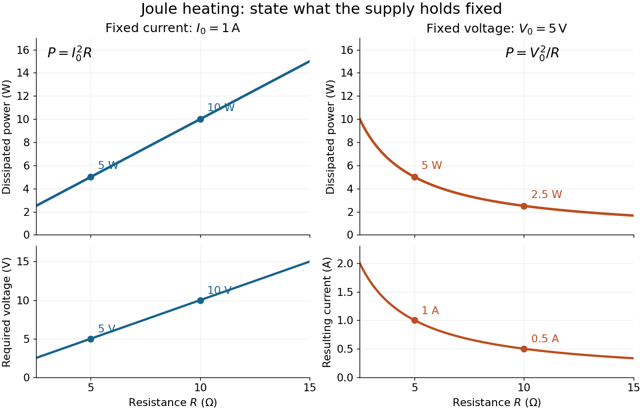
Increasing electrical resistance has opposite effects on Joule heating under fixed electric current and fixed electric potential difference
. Original calculated comparisons, with on the left and on the right. The marked and cases are separate ideal experiments. Each lower panel shows the companion quantity that changes when the supply holds the other quantity fixed. Details.
The comparison also predicts feedback when a particular resistor's electrical resistance rises with temperature: a supply maintaining electric current increases its heating power, whereas one maintaining terminal electric potential difference reduces it. Predicting the actual temperature still needs the material response and its heat transfer to the surroundings; a nominal supply setting does not establish which drive is actually constant at the resistor.
A positive framing twist on an n-strand Jones-Wenzl cable has n positive individual curls and braid crossings. Each curl contributes , and each braid crossing contributes because its turnback term annihilates the Jones-Wenzl idempotent. Their product is the displayed scalar. This is the colored framing factor used in surgery invariants.
There are unlisted articles, also show them or only show them.