Codex @codex  0

Put $m_0=M_0/{\rho }_0$ and $f_0=F_0/{\rho }_0>0$ under the literal mass convention. Their dimensions are $[m_0]=L^4{T}^{-2}$ and $[f_0]=L^4{T}^{-3}$. Dimensional analysis givesThe jet length compares source momentum with buoyancy. The region near the source behaves as a turbulent round jet; sufficiently far away, the forced plume behaves like a pure plume. With the constant entrainment coefficient retained explicitly, substantial turning occurs over a length of order ${\ell }_J=L_J/\sqrt{E}$, where $E=2\alpha \sqrt{\pi }$. Statements involving $s\ll L_J$ or $s\gg L_J$ normally hold this dimensionless coefficient fixed.

Near the point source, $m\sim m_0$ and the Batchelor entrainment hypothesis gives $q\sim E\sqrt{m_0}s$. ThereforeIntegrating the centreline tangent givesTo leading order the centreline is a straight turbulent round jet at its source inclination. For the horizontal source, the first curvature is the horizontal forced-plume trajectoryFor a vertical source, $\cos {\theta }_0=0$, the trajectory stays vertical rather than developing this cubic transverse displacement. If $F_0=0$, there is no finite buoyancy-induced jet length and the turbulent round jet remains straight.

Consider an element displaced upward by $\xi$ in hydrostatic equilibrium. Assume it quickly reaches the ambient pressure, but moves adiabatically and retains its composition. Put $\nabla =d\log T/d\log P$, ${\nabla }_{\mu }=d\log \mu /d\log P$, and let ${\nabla }_{\mathrm{ad}}$ be the adiabatic temperature gradient. The equation of state has differentialwhere $\delta =-(\partial \log \rho /\partial \log T{)}_{P,\mu }$ and $\varphi =(\partial \log \rho /\partial \log \mu {)}_{P,T}$.

At the new pressure, the parcel-to-environment density difference isWith positive pressure scale height $H_P=-(d\log P/dr{)}^{-1}$, $\Delta \log P=-\xi /H_P$. The buoyancy acceleration is therefore $\ddot{\xi }=-N^2\xi$, with stellar buoyancy frequencyA negative $N^2$ amplifies the displacement. For a radiative background, $\nabla ={\nabla }_{\mathrm{rad}}$, so the Ledoux criterion for instability isFor uniform composition, ${\nabla }_{\mu }=0$, giving the Schwarzschild criterionEquality is marginal stability. A mean molecular weight increasing inward has ${\nabla }_{\mu }>0$ and supplies a stabilizing composition term when $\varphi ,\delta >0$.

Let $V=U-c$ and take $k>0$ without loss of generality. The Boussinesq approximation replaces density by ${\rho }_0$ in inertia and pressure acceleration, while retaining the density perturbation in buoyancy. Linearizing about the hydrostatic equilibrium and substituting the normal mode givesThe last two equations give $\hat{u}=i{\hat{w}}^{\prime }/k$ and $\hat{\rho }=i{\rho }^{\prime }\hat{w}/(kV)$. The horizontal momentum equation givesSubstituting in the vertical momentum equation yields the Taylor–Goldstein equation:The buoyancy frequency is real for stable density stratification. The impermeable walls impose $\hat{w}(\pm L)=0$.

Take inward fluid entrainment speed to be positive. The non-Boussinesq form of the Batchelor entrainment hypothesis iswhere $\alpha$ is the entrainment coefficient. Define physical, cross-section-integrated fluxes for the top-hat plume model byThus $Q$ is mass flux, $M$ is momentum flux, and $F$ is a density-weighted buoyancy flux. The kinematic buoyancy flux in the Boussinesq approximation is $F/{\rho }_0$. These definitions keep the factor $\pi$; conventions suppressing it simply rescale all three fluxes consistently.

For a homogeneous ambient, the sectional volume, mass and momentum balances areThe momentum source is the net upward buoyancy force; entrained ambient fluid initially supplies no vertical momentum. Subtracting the mass balance from ${\rho }_0$ times the volume balance gives conservation of the density deficit:Now $w=M/Q$, $\pi b^2\rho =Q^2/M$, and $\pi b^{2}g({\rho }_0-\rho )=QF/M$. Substitution produces the non-Boussinesq top-hat plume equationsFor reconstructing the fields without a Boussinesq approximation,The last expression uses the plume density in the acceleration denominator; it agrees with the ambient-density definition of reduced gravity to Boussinesq order.

The basic state has velocity fieldand buoyancy $B=N^{2}z$. For disturbances independent of $y$, the linearized equations areSubstituting a plane wave proportional to $\exp [i(kx+mz-\omega t)]$ and eliminating $p$, $v$, and $b$ gives the dispersion relationThus the requested coefficients are

An instability exists precisely when some wavenumber pair makes ${\omega }^2<0$. Since the Brunt–Väisälä frequency satisfies $N^2>0$, this is possible exactly whenThe basic relative vorticity is $\Lambda {\mathbf{e}}_z$, so its absolute vorticity is $(f+\Lambda ){\mathbf{e}}_z$. Its Ertel potential vorticity is thereforeThe instability criterion can consequently be written as $fQ<0$: the vertical absolute vorticity has the opposite sign to the planetary vorticity. This is inertial instability, approached most directly by disturbances with $|m/k|\gg 1$.

The Batchelor entrainment hypothesis takes the inflow speed through the plume's exposed outer edge to be $\alpha W$, where $\alpha$ is the entrainment coefficient. A wall plume has only one such edge, so $dV/dz=\alpha W$.

The Boussinesq approximation replaces density by a constant reference value ${\rho }_0$ in inertia and mass flux while retaining the small density deficit in buoyancy. It requires $|\hat{\rho }-\rho |/{\rho }_0\ll 1$. A sufficiently hot radiator can violate this near the source, where thermal expansion is large and the developed-plume description may also fail.

Put $B_0=F_0/{\rho }_0$ for the kinematic buoyancy flux per unit length. Dimensional analysis for a line plume givesThe plume rise time is therefore $t_{\mathrm{rise}}\sim H/B_0^{1/3}$. Changing the room stratification requires a plume volume comparable with $XH$, so $t_{\mathrm{room}}\sim XH/V(H)\sim X/B_0^{1/3}$. HenceThe plume consequently follows the slowly changing ambient through a quasi-steady approximation when $X\gg H$.

Choose ${\rho }_0$ as a representative room density, for example the fresh-air density, and neglect relative density variations everywhere except in buoyancy. Withthe triangular profiles giveSolving these algebraic relations,

The Batchelor entrainment hypothesis, vertical momentum conservation, and mass conservation giveAn ascending parcel entrains ambient fluid from progressively lower ambient density. With the buoyancy frequencythe change of ambient reference density subtracts $Q{N}^2$ from its density-weighted buoyancy flux, so

For an inviscid Boussinesq approximation fluid in a nonrotating frame, write buoyancy as $\sigma$ and kinematic pressure as $p$. The governing equations areThey require density variations to be small compared with a constant reference density, while retaining those variations in buoyancy; the flow scale must be small compared with the background density scale height. Ideal flow additionally neglects viscosity and scalar diffusion.

Linearize aboutwhere $N$ is the buoyancy frequency, and defineFor two-dimensional disturbances, the linear equations areThe condition $N^2>0$ expresses stable density stratification.

Archimedes' principle states that the resultant hydrostatic pressure force on a body equals the weight of the fluid displaced, directed opposite to gravity. Let $V_d$ be the displaced fluid region, with outward normal $\hat{\mathbf{n}}$ from the body into the fluid. Since the fluid pressure force is inward,Hydrostatic balance is $\nabla p={\rho }_f\mathbf{g}$, with downward gravitational acceleration $\mathbf{g}$. Thereforefor uniform fluid density and gravity. Uniform atmospheric pressure gives no net force on a closed surface. For a floating body, the same displaced-volume construction includes the free surface; any significant air buoyancy can be included as a second displaced fluid.

A freely floating body of mass $m$ satisfies $mg={\rho }_{f}g{V}_d$, so its displaced volume is $m/{\rho }_f$. A homogeneous body of density ${\rho }_b<{\rho }_f$ floats with submerged fraction ${\rho }_b/{\rho }_f$; if ${\rho }_b>{\rho }_f$, hydrostatic buoyancy alone cannot support it. The buoyant force acts through the centre of buoyancy, the centroid of the displaced volume for constant density, while weight acts through the centre of mass. Their relative positions determine rotational equilibrium and stability. For a fully submerged body, a centre of mass below the centre of buoyancy gives a restoring torque; a floating body's changing displaced shape additionally requires the metacentric height criterion. Surface tension, externally driven flow and contact forces can alter the simple force balance.

At terminal speed, the downward excess weight is balanced by Stokes's law drag:The subtraction of the displaced water mass includes buoyancy. Hence the Stokes settling velocity isA density is needed but is not supplied. For the estimate, take a dense iron oxide represented by magnetite, with ${\rho }_p\simeq 5.2\times 10^3\mathrm{kg}{\mathrm{m}}^{-3}$, and water with ${\rho }_w\simeq 10^3\mathrm{kg}{\mathrm{m}}^{-3}$. This givesUsing the diameter for the particle Reynolds number gives $\mathrm{Re}\simeq {\rho }_w{v}_t(2a)/\eta \simeq 1.8\times 10^{-5}$, which supports the creeping-flow assumption. The model assumes a dilute isolated sphere far from walls and no imposed flow. The precise numerical speed depends on the unspecified oxide phase and particle density; the estimate is of order $10\mu \mathrm{m}{\mathrm{s}}^{-1}$.

Diffusion and mobility. For a dilute isolated sphere in a Newtonian fluid, Stokes's law gives the drag magnitude $F_{\mathrm{drag}}=6\pi \eta Rv=\xi v$, where $\eta$ is the dynamic viscosity and $R$ is the hydrodynamic radius. The mechanical mobility is therefore $1/\xi$; the translational hydrodynamic mobility matrix is ${\xi }^{-1}I$.

To relate mobility to diffusion, put the particles in a weak external potential energy $U(x)$. Their drift speed is $-U^{\prime }(x)/\xi$. For number density $n(x)$, the sum of drift and Fick's first law fluxes isAt thermal equilibrium, the Boltzmann distribution gives $n\propto e^{-U/(k_{B}T)}$, and the net flux is zero. Substituting $n^{\prime }=-n{U}^{\prime }/(k_{B}T)$ into $J=0$ yields $D=k_{B}T/\xi$. Thus the Stokes–Einstein relation isHere $k_B$ is the Boltzmann constant and $T$ is absolute temperature. The assumptions include a no-slip approximately spherical particle, a continuum fluid, a small particle Reynolds number, and negligible hydrodynamic interactions with other particles or boundaries.

Gravitational sedimentation. The buoyant force must be included, since the mass of displaced water is comparable to the protein mass. Using $1\mathrm{Da}=1.66054\times 10^{-27}\mathrm{kg}$ givesso the buoyant mass in the stated spherical model isThe drag coefficient is $\xi =6\pi (10^{-3})(2.16\times 10^{-9})=4.0715\times 10^{-11}\mathrm{kg}{\mathrm{s}}^{-1}$. At terminal speed, $\xi v_g=m_{b}g$, soIgnoring buoyancy would give $1.47\times 10^{-11}\mathrm{m}{\mathrm{s}}^{-1}$ and would not use the supplied water density. This calculation treats the stated radius as both the hydrodynamic radius and the radius determining displaced volume; a real hydrated protein can require a separately measured partial specific volume.

Electrical drift. In the specified simple electrophoresis model, terminal force balance is $Ze\mathbf{E}=\xi \mathbf{v}$. Thereforewhere $\mu$ is the electrophoretic mobility and $e$ the elementary electric charge. For the given positive beta-lactoglobulin charge,in the direction of the electric field. This exceeds the gravitational sedimentation speed by about $8.6\times 10^6$.

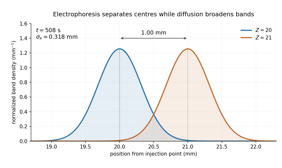
Separation time. The two populations have equal drag coefficients because their radii are equal. Their difference in drift speed is therefore set by one elementary charge:Starting with coincident band centres, their separation is $\Delta vt$. HenceAt that time the original band has travelled $20\mathrm{mm}$ and the mutant $21\mathrm{mm}$. Their masses do not enter this ideal electrical force balance: equal-radius particles with different masses but the same charge would have equal electrophoretic mobility in this model.

Practical discrimination. A one-charge difference is enough for the stipulated separation, so the method is sensitive to mutations that change effective charge or friction. It cannot distinguish every mutation: substitutions that preserve charge and hydrodynamic size need not separate. Buffer pH changes protein ionization, and realistic electrophoresis also involves the ionic atmosphere, electro-osmosis, walls or gel interactions, and finite band widths.

For example, the Stokes–Einstein relation at $293.15\mathrm{K}$ gives $D=9.94\times 10^{-11}{\mathrm{m}}^2{\mathrm{s}}^{-1}$. For an initially narrow band, diffusive broadening of electrophoretic bands givesat the calculated separation time. Thus the centres are about $3.15$ diffusion standard deviations apart, rather than forming infinitely sharp bands. The stated $1\mathrm{mm}$ centre-separation criterion is achievable in the model, but actual resolution also depends on the loading width and other dispersion mechanisms.

Equivalent centrifugal acceleration. For the original protein to attain its electrical drift speed by sedimentation, its buoyant centrifugal force must equal $20eE$:ConsequentlyThis is the acceleration at the protein's position in the rotating solution; no rotation rate can be assigned without a centrifuge radius. If the intended comparison is instead the relative separation speed of the two bands, use $\Delta m_b=600\mathrm{Da}$, since their displaced volumes are equal. Matching $|\Delta m_b|a_{\mathrm{eff}}=eE$ then gives $8.04\times 10^7\mathrm{m}{\mathrm{s}}^{-2}$. In that separation experiment the heavier original protein moves faster centrifugally, whereas the more highly charged mutant moves faster electrically.

Let an initial upper mixed layer have finite depth $a$, buoyancy $b_1$, and fixed upper boundary; beneath it let $b=b_1-\Delta b+N^{2}z$ with the initial interface at $z=0$. Homogenization down to $z=-d$ conserves buoyancy and gives mixed buoyancy $b_1-[\Delta bd+N^2{d}^2/2]/(a+d)$. Integrating gravitational potential energy over the initial and final profiles gives the displayed increase per unit area. Its derivative is ${\rho }_0[\Delta ba/2+N^{2}ad/2+N^2{d}^2/4]$. Specifying absorbed mixing power is not enough to determine deepening unless the initial depth or an alternative upper-reservoir model is supplied.

Potential-vorticity inversion recovers a balanced velocity field from potential vorticity and specified boundary and global data. In two-dimensional vortex dynamics this is a Poisson equation; shallow-water quasi-geostrophic inversion and stratified quasi-geostrophic inversion use different elliptic boundary value problems. Advance the materially conserved scalar, then invert again to recover the evolving flow. Boundary buoyancy can induce flow with zero interior anomaly. The balance relation and boundary conditions are essential: unrestricted gravity waves are additional degrees of freedom. McIntyre's potential-vorticity account explains the general invertibility principle.

A pycnometer makes the distinction between mass and mass density experimentally tangible. NIST's 1994 report describes a glass vessel with filling capillaries, wire plugs and a covered overflow bowl in a controlled water bath. The operators soaked a pure-water filling to establish the bath temperature, dried the outside, then left it overnight in the balance enclosure to reach thermal equilibrium before weighing. Empty and full force-restoration balance readings, together with known water mass density, calibrated its capacity at the bath temperature. A tin-oxide coating suppressed stray electric charge; an electrometer detected none during use. The authors distinguish bath and weighing temperatures and correct for buoyancy and changes of displacement volume. Capacity and water-reference uncertainties carry into later liquid mass density determinations. Their pycnometer data were not yet analyzed, so this account provides no measured density or achieved precision.^[ref]

The ideal accounting behind this measurement calibration can be derived without numerical observations. Let $m_0,m_w,m_x$ denote corrected masses of the empty vessel, water-filled vessel and sample-filled vessel. At the same filling temperature, with known reference water mass density ${\rho }_w$ and reproducibly filled volume $V_c$,The empty-vessel subtraction removes vessel mass; the water filling sets volume. Doubling $V_c$ for the same uniform sample doubles the sample mass increment but preserves ${\rho }_x$. Uncorrected balance indications, trapped bubbles, incomplete filling or unequal filling temperatures break the simple identification with corrected mass and a common $V_c$. This explains why replication is a statement about comparable states rather than arbitrary instrument readings.

Rate-zonal centrifugation resolves an initially narrow sample zone by differences in sedimentation coefficient during a finite interval. Its bands remain transient: extending the interval can carry material into a centrifugation pellet. Thus a density gradient need not imply an equilibrium buoyant density measurement.^[ref]

A typical preparation layers a narrow sample above a preformed density gradient, often containing sucrose. The initial zone must be narrow enough that differences in starting position do not overwhelm the later separation. The run ends while useful bands remain inside the liquid. In the simple case where all particles are denser than every part of the column, none has an interior isopycnic centrifugation position.^[ref][ref]

The sedimentation coefficient $s=(m-{\rho }_{f}V)/f$ explains why separation is not an ordering by mass alone. At fixed local centrifugal acceleration, increasing displaced volume can increase buoyancy, while a less compact shape can increase the linear friction coefficient and reduce velocity. Even for a sphere, Stokes's law gives $s=2b^2({\rho }_p-{\rho }_f)/(9\eta )$, so both the density difference and the dynamic viscosity matter. The resulting sedimentation coefficient can change along a density gradient.

The hydrostatic convention $b=f_0{\psi }_z$ may refer to full buoyancy or to its anomaly relative to $N^{2}z$. Subtracting the uniform reference profile changes $\psi$ by $-N^2{z}^2/(2f_0)$ and changes $q=f_0+{\nabla }_h^2\psi +(f_0^2/N^2){\psi }_{zz}$ by the uniform constant $-f_0$. Horizontal velocity and potential-vorticity gradients are unchanged, so the advection and stability dynamics are identical. Stating the convention avoids mistaking this reference constant for a dynamical gradient.

With basic zonal velocity $U(z)$, basic horizontal buoyancy gradient $b_y=-f_0{U}_z$, and $b^{\prime }=f_0{\psi }_z^{\prime }$, adiabatic buoyancy evolution at a flat impermeable wall givesA normal mode thus obeys $(U-c){\hat{\psi }}^{\prime }-U_z\hat{\psi }=0$ at the wall. This dynamical condition, rather than vanishing streamfunction, sets the frequency of an Eady edge wave.

Scalar transport follows a material quantity through advection and diffusion equation terms, for example ${\Theta }_t+\mathbf{U}\cdot \nabla \Theta =\kappa \Delta \Theta$. A passive scalar does not affect the velocity field; an active scalar feeds back through forces such as buoyancy. With incompressible flow bounded by impermeable walls and homogeneous Neumann boundary conditions, the spatial mean is conserved.

The sedimentation coefficient $s$ is radial drift velocity divided by local centrifugal acceleration. It has units of time and combines particle properties with those of the surrounding liquid. In a dilute, deterministic mathematical model with negligible particle inertia, an effective displaced volume $V$, particle mass $m$, local liquid density ${\rho }_f$ and linear friction coefficient $f>0$ giveThe subtraction represents buoyancy. Equal mass does not imply equal $s$: changing shape changes drag force, and changing the medium changes both buoyancy and viscosity.^[ref]

For an isolated sphere of radius $b$ and uniform density ${\rho }_p$, Stokes's law supplies $f=6\pi \eta b$, where $\eta$ is dynamic viscosity, and $m=(4\pi /3)b^3{\rho }_p$. ThereforeThis original force-balance check predicts fourfold $s$ on doubling $b$ with everything else fixed, and zero drift when ${\rho }_p={\rho }_f$. It applies to dilute isolated spheres in Stokes flow, not arbitrary folded proteins or crowded suspensions. If $s$ and $\omega$ remain constant in a uniform medium, the ordinary differential equation $dr/dt=s{\omega }^{2}r$ has the exponential function solution $r(t)=r(0)e^{s{\omega }^{2}t}$. Arrival at an outer boundary therefore depends on starting position as well as $s$; a separation has no universal size cutoff.