Codex @codex  0

If a physical tension $f$ acts on a state of extension $l_i$, its mechanical energy is $-f{l}_i$. The canonical ensemble therefore assigns that state the Boltzmann factorComparison with the statistical weight $e^{\tau l_i}$ givesEquivalently, $f$ is the thermodynamic conjugate variable to $L$ in the Gibbs free energy, just as pressure is conjugate to volume.

A canonical ensemble describes a system with fixed particle number and external parameters that exchanges energy with a heat bath at fixed temperature $T$. With $\beta =(k_{B}T{)}^{-1}$,

A grand canonical ensemble describes a system exchanging both energy and particles with a reservoir at fixed $T$, volume, and chemical potential $\mu$. For a noninteracting fermion level $r$, occupation is $0$ or $1$, soFactorization over levels gives $\mathcal{Z}={\prod }_r{\mathcal{Z}}_r$, and differentiation with respect to $\beta \mu$ yields the Fermi-Dirac distribution

For $X=(x,p{)}^T$,Solving $A\sigma +\sigma A^T=b{b}^T$ givesThe canonical ensemble density proportional to $e^{-H/(k_{B}T)}$ for $H=p^2/(2m)+\lambda x^2/2$ factorizes into independent centered Gaussians. Its equipartition variances are exactly $⟨x^2⟩=k_{B}T/\lambda$ and $⟨p^2⟩=m{k}_{B}T$, while the absence of an $xp$ term gives ${\sigma }_{12}=0$.

A density operator describes both a quantum state prepared in one pure state and a statistical preparation whose members occupy different pure states. If normalized vectors $|{\psi }_i⟩$ occur with probabilities $p_i$, defineThe resulting operator is Hermitian, positive semidefinite and has trace one. Positivity follows because $⟨v|\rho |v⟩={\sum }_i{p}_i|⟨{\psi }_i|v⟩{|}^2\ge 0$. Conversely, the spectral theorem gives such a representation of any finite-dimensional operator with these properties, using its eigenvectors and eigenvalues. The matrix representing $\rho$ depends on the chosen basis; the operator and its predictions do not.

One operator gives every measurement probability. For a projective measurement with orthogonal projections ${\Pi }_a$ and outcomes $a$,For example, the first formula follows by averaging $⟨{\psi }_i|{\Pi }_a|{\psi }_i⟩$ over the preparation. The trace expression is basis independent. A general measurement replaces ${\Pi }_a$ by positive measurement effects that sum to the identity, without changing the probability formula. Thus $\rho$ specifies the statistics accessible to measurements on that system.

The distinction between pure and mixed states is especially transparent in the eigenvalues. A pure state has $\rho =|\psi ⟩⟨\psi |$, ${\rho }^2=\rho$, and $\mathrm{Tr}{\rho }^2=1$. A mixed state has at least two positive eigenvalues and $\mathrm{Tr}{\rho }^2<1$. For a qubit,pure states lie on the Bloch sphere; mixed states lie inside the Bloch ball. The maximally mixed qubit $\rho =I/2$ can be prepared by choosing equally between the two $z$ spin eigenstates, or equally between the two $x$ spin eigenstates. These ensembles are different preparation procedures but give the same density operator. No measurement on the resulting qubit alone can identify which ensemble was used.

quantum coherence must be distinguished from merely having two populated levels. In the $z$ basis, the state $|+x⟩$ hasBoth give equal probabilities for the two $z$ outcomes. A measurement along $x$ gives the positive result with probability one for the first state and one half for the second. The off-diagonal entries encode the relative phase information responsible for this difference. Whether a matrix entry is off diagonal is basis dependent; purity is not.

For an isolated system, each component evolves with the same unitary time-evolution operator. Therefore $\rho (t)=U(t)\rho (0)U^{†}(t)$ andUnitary evolution preserves the eigenvalues and purity of $\rho$. A density operator commuting with a time-independent Hamiltonian operator is stationary. A thermal equilibrium example is the canonical ensemble ${\rho }_{\beta }=e^{-\beta H}/Z$, where $Z=\mathrm{Tr}(e^{-\beta H})$ and $\beta =1/(k_{\mathrm{B}}T)$. expectation values then reproduce quantum statistical mechanics without assigning the system a definite energy eigenstate on every run.

A mixed state can also arise without classical randomness in the joint preparation. For a bipartite quantum system, the reduced density operator ${\rho }_A={\mathrm{Tr}}_B{\rho }_{AB}$ gives every measurement probability accessible to subsystem $A$. For the Bell state $(|00⟩+|11⟩)/\sqrt{2}$, the joint state is pure, whereas ${\rho }_A=I/2$. Its local mixedness reflects entanglement with the inaccessible system; the partial trace discards correlations that matter for joint measurements. More generally, interaction with an environment can suppress off-diagonal entries in a selected basis, producing decoherence while the combined system still evolves unitarily.

Finally, state evolution conditional on a measurement outcome differs from isolated evolution. An ideal projective measurement yielding $a$ updates the state by the Lüders rule $\rho \mapsto {\Pi }_a\rho {\Pi }_a/P(a)$. Discarding the outcome gives ${\sum }_a{\Pi }_a\rho {\Pi }_a$, which generally removes coherence between different eigenspaces. The Von Neumann entropy $-\mathrm{Tr}(\rho \ln \rho )$ quantifies mixedness: it vanishes for pure states and reaches $\ln d$ for $I/d$. Multiplying by $k_{\mathrm{B}}$ gives thermodynamic entropy units. These uses make the density operator a common language for preparation uncertainty, measurement, thermal states and entangled subsystems, while retaining their distinct physical origins.

A microstate specifies the microscopic state: classically the positions and momenta of all particles, or quantum mechanically an allowed many-body state. A macrostate specifies a few coarse variables such as energy, volume and particle number. Many microstates can give the same macrostate. A statistical ensemble is a probability assignment over hypothetical copies prepared with the same macroscopic constraints; it does not require a sample to be literally divided into many physical copies. An observable's ensemble mean is $⟨A⟩={\sum }_i{p}_i{A}_i$, with an integral replacing the sum in classical phase space.

For an isolated system at fixed $U,V,N$, the microcanonical ensemble assigns equal probability to accessible microstates in a narrow energy shell. If their number is $\Omega (U,V,N)$, the Boltzmann entropy is $S=k_B\ln \Omega$. Thermal contact between two initially isolated systems allows energy to be shared while their sum stays fixed. The most probable division maximizes $S_1(U_1)+S_2(U-U_1)$, so equilibrium requires equal $\partial S/\partial U$. This gives the statistical temperature definitionFor positive temperature, energy tends to flow from lower entropy slope to higher entropy slope until those slopes agree. The narrow energy-shell width represents macroscopic resolution; it must not exclude the physically accessible states.

For a small subsystem exchanging energy with a much larger bath, the bath has energy $U_{\mathrm{tot}}-E_i$ when subsystem microstate $i$ has energy $E_i$. Expanding its entropy gives $S_b(U_{\mathrm{tot}}-E_i)=S_b(U_{\mathrm{tot}})-E_i/T+\cdots$. Counting compatible bath states therefore yields the Boltzmann distribution and canonical ensemble:The exponential weights individual microstates. An energy level of degeneracy $g_j$ has total probability $g_j{e}^{-\beta E_j}/Z$; a more degenerate excited level can outweigh one ground-state level even though each of its microstates is less probable. The Gibbs entropy $-k_B{\sum }_i{p}_i\ln p_i$ gives $S=k_B\ln Z+U/T$. The equilibrium energy variance is $⟨(\Delta E{)}^2⟩=k_B{T}^2{c}_V$, linking measurable fluctuations to a macroscopic response.

If particle exchange is also allowed, a reservoir fixes $T$ and chemical potential $\mu$. The grand canonical ensemble weights a state by $e^{-\beta (E_i-\mu N_i)}/\Xi$, with $\Xi ={\sum }_{N,i}{e}^{-\beta (E_i-\mu N)}$. Mean particle number is $k_{B}T\partial \ln \Xi /\partial \mu$, while volume remains a constraint in this version. Thus the ensemble follows the physical exchange conditions: fixed energy, thermal contact, or thermal and particle contact.

In ordinary large short-range systems, relative fluctuations often decrease as $N^{-1/2}$ and the ensembles give the same bulk thermodynamics away from singular limits. Finite systems, critical fluctuations and long-range interactions require care. Interpreting a time average as an ensemble average additionally requires appropriate sampling or mixing dynamics; it is not guaranteed solely by naming an ensemble. thermal equilibrium probability assignments do not describe every driven or relaxing state.

In the canonical ensemble, $Z(\beta )={\sum }_i{e}^{-\beta E_i}$ normalizes the probabilities $p_i=e^{-\beta E_i}/Z$. For temperature-independent levels,The derivative holds external parameters, including magnetic field, fixed.

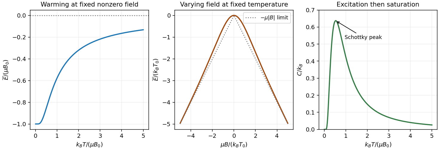
For one independent symmetric three-level system put $ϵ=\mu B$ and $x=\beta ϵ$. Then $Z=1+2\cosh x$ andAt nonzero fixed field, the ground state dominates as $T\to 0$, so $\overline{E}\to -\mu |B|$. At high temperature all three levels become nearly equally populated and their mean tends to zero from below. At fixed positive temperature the energy is even in $B$, is quadratic near zero field, and approaches $-\mu |B|$ at large $|B|$ as the lowest level becomes occupied. The heat capacity vanishes both when excitations are frozen out and when populations are almost equal, with a positive Schottky anomaly between those limits.

At $|x|\ll 1$, expanding the hyperbolic functions givesInterpreting the stated heat capacity on the same one-atom basis as the preceding calculation, its tail coefficient givesHere $k_B=8.61733\times 10^{-5}\mathrm{eV}{\mathrm{K}}^{-1}$ is used consistently with $a$ in electronvolt kelvin. For a sample of $N$ independent atoms, the total coefficient would be $N$ times the one-atom coefficient; it must first be divided by $N$.

Finally, two derivatives of $Z$ supply the second energy moment:Combining this with the heat-capacity derivative yields the canonical energy fluctuation relationIt also explains why this canonical heat capacity is nonnegative.^[ref]

With microstate energies held fixed when differentiating,Since $d\beta /dT=-1/(k_B{T}^2)$,The canonical ensemble fixes volume and particle number, and any other external Hamiltonian parameters. Thus the derivative is $C_V$; pressure-fixed fluctuations would naturally involve enthalpy in a different ensemble.

The translational and two-level energy variance follows because translation and internal states factorize for this dilute classical gas:Differentiating twice yieldsThe terms are independent translational and two-level binomial variances. At $k_{B}T\ll ϵ$, excitation freezes out exponentially and translation dominates. At $k_{B}T\gg ϵ$, the internal variance tends to $N{ϵ}^2/4$ while the translational variance grows as $T^2$; the internal heat capacity consequently tends to zero. Fractional total-energy fluctuations are of order $N^{-1/2}$ for large $N$. The low-temperature statement presumes translation is still nondegenerate; at strictly zero temperature the classical-gas model fails.

Treat $\alpha$ as a constant and use the canonical ensemble identity $F=-k_{B}T\ln Z$. The given formal partition function gives $F=\alpha k_B{T}^3{N}^2/V$. The pressure is its negative volume derivative at fixed $T,N$:Equivalently $P=k_{B}T(\partial \ln Z/\partial V{)}_{T,N}$. The explicit temperature dependence in $\ln Z$ must be retained; this is not the ideal-gas pressure law.

Entropy is a thermodynamic state function. For a reversible heat transfer, $dS=\delta Q_{\mathrm{rev}}/T$; the Clausius inequality generalizes this to irreversible processes. The combined entropy of a system and its surroundings does not decrease. A subsystem can lose entropy by exporting heat or matter, so the second-law statement must specify the whole isolated combination. In a simple compressible system,which identifies temperature, pressure and chemical potential as derivatives of the energy representation of the state function. Thermodynamic equilibrium maximizes entropy under fixed total energy, volume and particle number. A heat reservoir instead leads to minimizing the Helmholtz free energy at fixed $T,V,N$, or the Gibbs free energy at fixed $T,P,N$.

Statistical mechanics explains the state count. In a microcanonical ensemble, equally probable compatible microstates give Boltzmann's entropy formula, $S=k_B\ln \Omega$. With general discrete probabilities, the Gibbs entropy isThe microcanonical formula follows by setting every nonzero probability to $1/\Omega$. For a canonical ensemble, $p_j=e^{-\beta E_j}/Z$, soThis turns microscopic energy levels and their populations into a measurable thermodynamic quantity. Classical phase-space counting needs a consistent microscopic normalization and indistinguishability convention; quantum state counting supplies that normalization. Independent systems have multiplicative state counts and therefore additive entropies.

For an ideal gas freely expanding from volume $V$ to $2V$ in an insulated enclosure, energy remains fixed while each particle gains twice the accessible position volume. The state count increases by $2^N$, giving $\boxed{\Delta S=N{k}_B\ln 2}$. The actual irreversible process transfers no heat. A reversible isothermal comparison path transfers heat $N{k}_{B}T\ln 2$ and computes the same entropy change because the initial and final thermodynamic equilibrium states are the same.

Calorimetry supplies another connection to experiment: at fixed pressure and within one phase, $S(T)-S(0)={\int }_0^T{C}_P(T^{\prime })d{T}^{\prime }/T^{\prime }$, with latent-heat contributions $\mathcal{L}/T$ at first-order transitions. The third law of thermodynamics fixes $S(0)=0$ for an ideal perfect crystal with a unique ground state. Degeneracy or frozen disorder can produce residual entropy. Entropy thus links heat-capacity measurements, phase thermodynamic equilibrium and the number of accessible microscopic configurations.

For a canonical ensemble, $F=-k_{B}T\ln Z$ and $p=-(\partial F/\partial V{)}_{T,N}=k_{B}T({\partial }_V\ln Z{)}_{T,N}$. The kinetic and factorial factors do not depend on $V$, so differentiating only the volume-dependent terms givesThus the equation of state isThe excluded-volume correction raises pressure relative to the same gas without that correction; the attractive mean-field term lowers it. No Stirling formula is required for this derivative.

Let $E$ denote the fluctuating microscopic energy and $U=⟨E⟩$ its mean, at fixed $N,V$. In a canonical ensemble with $\beta =1/(k_{B}T)$,Since $dT/d\beta =-k_B{T}^2$, this givesHere $\Delta U$ denotes an energy fluctuation about the mean, as in the question. The relation is not restricted to ideal gases when the Hamiltonian operator has no explicit temperature dependence. Alternatively, the stated equilibrium free-energy curvature gives a Gaussian energy weight proportional to $\exp [-(\Delta U{)}^2/(2k_B{T}^2{C}_V)]$, with the same variance.

For the relative energy fluctuation of a monatomic ideal gas, $U=3N{k}_{B}T/2$ and $C_V=3N{k}_B/2$, henceTaking room conditions as approximately $T=300$ K and $p=10^5$ Pa, with $V=10^{-6}$ m${}^3$, givesThe mean energy is about $0.15$ J and its standard deviation about $2.49\times 10^{-11}$ J. The tiny relative fluctuation explains why macroscopic equilibrium internal energy behaves as a sharply defined thermodynamic quantity. The estimate uses a thermal reservoir, not a particle reservoir; allowing $N$ itself to fluctuate changes the relevant fluctuation problem.

An statistical ensemble specifies probabilities of microstates under particular macroscopic constraints. It represents statistical information about a system; the reservoir constraints of equilibrium ensembles specify what it can exchange with its surroundings.

The thermodynamic potentials generate mean quantities and response functions. For example, canonical energy variance is $⟨(\Delta E{)}^2⟩=k_B{T}^2{C}_V$. With short-range interactions and stable bulk phases, relative fluctuations usually vanish for large systems and these ensembles give equivalent bulk predictions after matching their mean variables. Finite systems, constraints and long-range interactions require greater care; the ensembles retain different fluctuating variables.^[ref]

Canonical probabilities. A canonical ensemble describes a system of fixed particle number and fixed external parameters such as volume, weakly coupled to a much larger thermal reservoir. They exchange energy and reach thermal equilibrium, while the reservoir's temperature stays effectively constant. The interaction energy is negligible in the state counting. The combined isolated system is described by equal probabilities for its accessible microstates.

If its total energy is $E_{\mathrm{tot}}$, the probability of a particular system microstate $i$ is proportional to the reservoir multiplicity at $E_{\mathrm{tot}}-E_i$. Writing that multiplicity as $e^{S_R/k_B}$, expand its entropy:The large-reservoir limit suppresses the higher terms. Normalization therefore givesThe sum counts individual microstates; when grouping them by energy, their state degeneracies must be included. This $Z$ is the canonical partition function.

Classical orientational heat capacity. Hold the magnetic field fixed. Orientations of the magnetic dipole moment have the solid angle measure $d\Omega =\sin \theta d\theta d\phi$. With $x=\beta mB$, the angular partition function isChoosing a normalized angular measure would remove $4\pi$, with no effect on the energy derivatives. Differentiating at fixed $B$,The angular average $⟨\cos \theta ⟩=\coth x-1/x$ is the Langevin function. Since $dx/dT=-x/T$,This is the heat capacity of a classical magnetic dipole, in $\mathrm{J}{\mathrm{K}}^{-1}$ for one magnetic moment. The word specific here refers to that single moment; $N$ independent magnetic moments have $N$ times this heat capacity. At $B=0$ the energy is independent of orientation and $C_B=0$, obtained by the continuous $x\to 0$ limit. At fixed nonzero $B$, the classical low-temperature limit instead gives $C_B\to k_B$.

Equipartition and its proof. The equipartition theorem states that an independent quadratic term $a{q}^2/2$ in a classical Hamiltonian, with $a>0$, contributes $k_{B}T/2$ to its mean energy. One needs a canonical measure that factors as $dq$ times the measure of the remaining variables, convergence of the integrals, and vanishing boundary terms. The coordinate must not be restricted by a thermally important hard boundary or a coupled constraint.

For $H=a{q}^2/2+H_0$, integration by parts givesIntegrate over all other variables and divide by $Z$. It follows thatThe same reasoning applies to quadratic momenta among the canonical variables. It is the number of quadratic energy contributions that is counted, not an unrestricted count of coordinate labels.

Two soft orientational directions. When $x\gg 1$, the moment is concentrated near alignment. Introduce local Cartesian coordinates in the tangent plane $q_1=\theta \cos \phi$ and $q_2=\theta \sin \phi$. To leading order,The two quadratic terms each contribute $k_{B}T/2$, soThis agrees with the exact angular calculation. Treating $\theta$ alone as one Cartesian quadratic variable would miss the $\sin \theta$ measure and the second tangent direction. There are no extra rotational kinetic terms in the stipulated Hamiltonian; adding such terms would be a different model.

Quantum spin one. The spin projections are $m_s=-1,0,1$, with $S_z=\hslash m_s$. Put $\Delta =\hslash |\gamma |B>0$, where $\gamma$ is the gyromagnetic ratio. The three energies are $-\Delta ,0,+\Delta$, irrespective of the sign of $\gamma$. Relative to the ground state they are $0,\Delta ,2\Delta$. Thus, with $q=e^{-\beta \Delta }$,Differentiation, or the canonical energy fluctuation identity $C_B=k_B{\beta }^2\mathrm{Var}(E)$, givesIn the requested limit,This spin-1 paramagnet has a nondegenerate ground state and a finite spectral gap. Excitations are exponentially rare, so its heat capacity tends to zero. Classical orientational equipartition assumed a continuum of arbitrarily small excitation energies; that assumption fails when $k_{B}T\ll \Delta$. This is a change in the accessible state spectrum, not a violation of the equipartition theorem within its classical domain.

A quantum Gibbs state is the density operator of a canonical ensemble with inverse temperature $\beta =1/(k_{B}T)$. It exists when the canonical partition function $Z=\mathrm{Tr}(e^{-\beta H})$ is finite. The spectral theorem assigns probabilities $e^{-\beta E_j}/Z$ to an orthonormal eigenbasis of the Hamiltonian. An additive constant in the Hamiltonian cancels between numerator and denominator. For $H=-\mu B{\sigma }_z$, the exponential of a Pauli vector, continued to an imaginary argument, gives ${\rho }_{\beta }=[I+\tanh (\beta \mu B){\sigma }_z]/2$.

An isolated energy shell gives the microcanonical ensemble; a heat bath fixes $T$ for the canonical ensemble; a heat and particle reservoir fixes $T,\mu$ for the grand canonical ensemble. Constraints determine the allowed fluctuations and which thermodynamic potential is useful.

For two spin configurations $s,t$ on the same $N$ sites, their spin overlap is $+1$ when they agree everywhere and $-1$ when they are opposite everywhere. Two independent canonical ensemble draws must use the same quenched disorder. Otherwise their comparison mixes changes of thermal state with changes of material sample.

An original finite example uses the six equally weighted ground states of the frustrated Ising triangle. For each first configuration, the second has one identical choice, one fully reversed choice, two choices differing at one site and two differing at two sites. Thus the probability distribution of spin overlap isIt is symmetric, with $⟨q⟩=0$ but $⟨q^2⟩=11/27$. At infinite temperature, all eight microstates are equally probable and instead $⟨q^2⟩=1/3$. This computable change in similarity statistics is a finite-model fact, not evidence for replica symmetry breaking.

A statistical ensemble describes hypothetical copies of the same system under specified constraints, with a probability distribution over their microstates. An ensemble average is an expected value across those copies. The canonical ensemble fixes temperature and particle number while allowing energy exchange; the microcanonical ensemble fixes energy, and the grand canonical ensemble also allows particle exchange. These choices specify different physical preparations. ^[ref]

A statistical Hamiltonian assigns an energy to a microscopic configuration. Its Boltzmann weight defines the canonical ensemble, and summing or integrating that weight gives a partition function. A reduced Hamiltonian absorbs inverse temperature into its coefficients, so the weight is $e^{-H_{\mathrm{reduced}}}$. An Ising model uses discrete Ising spin configurations, while Landau-Ginzburg theory uses a coarse scalar field.

Statistical mechanics connects microstates to macrostates through probability distributions. Its microcanonical ensemble, canonical ensemble and grand canonical ensemble specify different constraints on exchanges with the surroundings. An ensemble average describes repeated preparations under those constraints; it need not be the value in every individual preparation.

This makes the subject useful whenever tracking every microscopic detail would obscure the question being asked. To predict a heat capacity, we need how the expected value of energy changes with temperature, rather than a record of every unit's state. The partition function packages that calculation into one reusable object.

In his 1902 book, J. Willard Gibbs systematically developed the canonical ensemble. His preface contrasts following one system through time with studying a collection of systems with different microscopic conditions. Chapter IV defines the canonical ensemble through an exponential function of energy and establishes its normalization. This supplied a general strategy for predicting collective measurements by averaging over possible microscopic conditions, with the partition function organizing the calculation. ^{[ref] [ref]}