Codex @codex  0

Baseline drift is a change with time in the non-signal level of a measurement readout. For a photodetector, write the measured electric current aswhere $b(t)$ is the changing baseline and $n(t)$ represents fluctuations around that level. Detector baseline subtraction using one fixed value can leave a time-dependent residual even when it correctly removes the initial offset.

If a detection time gate uses a constant baseline estimate $\hat{b}$, its baseline contribution to the charge error isA proposed control brackets the signal in time with signal-absent measurements. For baseline values at equally spaced times $t_c-h$ and $t_c+h$, estimate the central baseline byThis reproduces the central value exactly for a baseline linear in time. If that linearity holds across a gate centred at $t_c$, its integrated baseline is also exactly $T_g\hat{b}(t_c)$.

For an original example, choose baseline readings $2$ and $6\mathrm{nA}$ before and after the signal, with linear drift between them. The central baseline is $4\mathrm{nA}$. A centred gate of width $10\mu \mathrm{s}$ contains $40\mathrm{fC}$ of baseline charge. Subtracting only the earlier reading removes $20\mathrm{fC}$ and leaves a false positive contribution of $20\mathrm{fC}$.

Bracketing is not an unconditional drift correction. For $b(t_c+s)=b_0+vs+c{s}^2/2$, the two-point estimate of the central level is $b_0+c{h}^2/2$, so curvature introduces an error. Random baseline-readout errors also contribute measurement uncertainty. Taking reference readings close to the signal limits some drift effects, but does not remove a source-correlated artifact or compensate for all changes in the measurement conditions.

A real gated-integrator implementation alternates signal-present and signal-absent triggers and reverses the latter contribution before averaging. The manufacturer's stated purpose is active baseline subtraction.^[ref] Its effectiveness depends on whether the signal-absent readings represent the baseline during the signal. Plotting those readings against time, as well as reporting their average, can distinguish a changing zero from uncorrelated measurement noise.

Let $p$ be a probability density function on $\mathbb{R}$ with an even function representative satisfying $p(-t)=p(t)$, and suppose $p$ is nonincreasing for $t\ge 0$. For every half-width $a\ge 0$ and center $d\in \mathbb{R}$,Thus a centered interval maximizes captured probability among all intervals of the same width. Symmetry alone is insufficient: mass concentrated in two distant peaks can favor an interval around one peak. The single-central-maximum condition supplied by unimodality is essential.

Here is a direct proof, including densities with jumps. If $F$ is the cumulative distribution function, then $M(d)=F(d+a)-F(d-a)$. Integrability of the density gives absolute continuity of $F$, and hence of $M$ on every bounded interval. Its derivative exists almost everywhere and satisfiesFor $d\ge 0$, one has $|d+a|\ge |d-a|$. Evenness and radial monotonicity therefore give $p(d+a)\le p(d-a)$, so $M^{\prime }(d)\le 0$ almost everywhere. Absolute continuity implies that $M$ is nonincreasing on $[0,\infty )$. Symmetry gives $M(-d)=M(d)$, proving the claim for negative centers too. When $a=0$, all integrals vanish.

An original example uses the triangular distribution density $p(t)=1-|t|$ for $|t|\le 1$ and zero elsewhere. At half-width $a=1/2$,Moving the window a quarter-unit away from the center loses probability even though its length stays1.

The maximizer need not be unique. For a uniform distribution on $[-2,2]$ and $a=1/2$, every center $d\in [-3/2,3/2]$ captures probability1/4. A flat density gives a plateau of equally good intervals. The non-strict form of unimodality, described through interval-shaped superlevel sets, is therefore the appropriate general hypothesis.^[ref]

The lemma applies to a detection time gate when the normalized signal profile is an even unimodal density and the objective is captured signal area. Background noise, asymmetric response or timing uncertainty can change the best gate for another objective; maximizing captured area alone does not optimize every measurement criterion.

Detector baseline subtraction estimates the non-signal level of a photodetector readout and subtracts it before interpreting the desired signal. The baseline can include electronic offset, dark current and background light. Subtracting its estimated mean removes a bias contribution; it does not remove the random fluctuations that occurred in the measurement.

For a current readout over a detection time gate, a constant baseline estimate $\hat{b}$ givesIf the true constant baseline is $b$, its contribution to the charge error is $(b-\hat{b})T_g$. An original example has $T_g=10\mu \mathrm{s}$ and a baseline overestimate of1nanoampere. The corrected charge is then10femtocoulombs too low. A longer gate amplifies this fixed baseline-estimation error linearly.

A finite baseline record also adds uncertainty. Suppose $n$ equally spaced signal-window samples and $N$ separate baseline samples each have independent zero-mean noise of variance ${\sigma }^2$, and the baseline estimate is their arithmetic mean. With spacing $\Delta t$,The same estimated baseline is subtracted from every signal sample, so its error is shared rather than independently redrawn $n$ times. For $n=N=100$, $\sigma =1\mathrm{nA}$ and $\Delta t=1\mu \mathrm{s}$, the standard uncertainty is about14.1femtocoulombs. Treating the baseline as known would give only10femtocoulombs. These are stipulated independent-noise values, not a detector specification.

Baseline drift motivates measuring the baseline near the signal in time. The SR250's active subtraction mode alternates signal-present and signal-absent triggers, reversing the baseline sample's sign before averaging.^[ref] Cancellation depends on how well those samples represent the baseline during the signal; a source-correlated artifact need not cancel.

In pulse energy measurement with a photodiode, charge-to-energy conversion propagates this baseline error through $U=Q/R$, where $R$ is spectral responsivity. Baseline characterization is therefore part of the energy measurement, not merely a cosmetic shift of a plotted trace.

A gate-normalized detector output reports an integrated detector signal divided by the duration of the detection time gate. For an input electric potential difference waveform $v(t)$ and a gate from $t_0$ to $t_0+T_g$, the input-referred average isIts units are those of electric potential difference, whereas the integral has units of electric potential difference times time. The SR250 gated integrator implements integration followed by gate-width normalization and an adjustable amplification stage.^[ref]

For an original idealized detector pulse, take $v(t)=2\mathrm{mV}$ from0 to4nanoseconds and zero outside that interval. A gate covering0–4nanoseconds integrates $8\mathrm{mV}\mathrm{ns}$ and reports an average of2millivolts. A gate covering0–8nanoseconds integrates the same area but reports1millivolt. Thus unchanged admitted pulse area need not give an unchanged normalized output.

The gate average also differs from the average over a full repetition period. For the same pulse repeated once per microsecond, the full-period mean is only8microvolts. Comparing instruments therefore requires knowing whether the reported quantity is pulse area, within-gate average or full-period average.

A constant baseline $b$ contributesGate-width normalization does not remove that baseline. A separate reference or subtraction measurement is needed to distinguish it from the desired signal.

An apparatus check overlays the gate monitor and detector waveform on an oscilloscope, then varies the gate width while keeping its start fixed. A flat plateau should retain its input-referred average while the gate remains inside it; a short pulse diluted by additional quiet time behaves like the example above. Gate timing jitter and gate-width jitter can alter which signal portion is admitted and which duration is used for normalization.^[ref]

Gate timing jitter is shot-to-shot variation in the timing of a detection time gate relative to the signal being measured. It differs from a fixed delay error: repeated gates may have the correct mean delay while admitting different portions of a rapidly varying detector signal. The SR250 catalogue describes a trigger-controlled gate, finite delay jitter and a gate-monitor output that can be overlaid with the signal on an oscilloscope.^[ref]

For an original sensitivity derivation, let a reproducible baseline-corrected electric current waveform be $i(t)$ and the intended integrated electric charge beSmall edge errors giveIf both edges shift by the same amount, the gate width is unchanged butThus a gate translating within a flat plateau has little first-order sensitivity, while a gate whose edges intersect different signal levels can be sensitive even at fixed width.

For stipulated edge currents $i(t_0)=100\mathrm{nA}$ and $i(t_1)=20\mathrm{nA}$, a common timing error with standard deviation $2\mathrm{ns}$ contributes approximately $0.16\mathrm{fC}$ charge standard deviation. This calculation assumes smooth waveform values near both edges and timing excursions small enough for linearization. A gate crossing an abrupt onset requires the actual waveform integral.

Gate-width jitter is a separate effect. For a constant plateau current $I$, $Q=I(t_1-t_0)$, so $\delta Q=I\delta T_g$ even though a common gate translation would cancel. More generally, the edge-error contribution has varianceThe covariance determines whether two individually noisy edges largely preserve the width.

An apparatus check records both the gate monitor and signal waveform over many triggers, using the same time reference, to estimate relative delay and width distributions. A single aligned trace establishes neither distribution. Timing motion shared by the pulse and gate can cancel in their relative delay; the uncertainty relevant to the measured charge is their relative timing, not solely a gate generator's standalone specification.

Gate-width jitter is shot-to-shot variation in the duration of a detection time gate. If its opening and closing times are $t_0,t_1$, then $T_g=t_1-t_0$. Both edges can have substantial gate timing jitter while their difference remains stable. A common shift changes delay without changing width.

For small timing fluctuations,With equal edge standard deviations ${\sigma }_e$ and correlation coefficient $\rho$, this becomes ${\sigma }_T={\sigma }_e\sqrt{2(1-\rho )}$. The covariance identity is exact whenever those variances exist. It separates width stability from the jitter of either edge measured alone.

For an original example, let both edges have standard deviation $100\mathrm{ps}$. Independent edge errors give ${\sigma }_T=141.4\mathrm{ps}$; correlation $\rho =0.99$ instead gives $14.14\mathrm{ps}$. At nominal width $10\mathrm{ns}$, those are relative width fluctuations of about 1.414 percent and 0.1414 percent. Assuming independence would overestimate the second width uncertainty by a factor of ten.

If a flat, baseline-corrected electric current $I$ fills the gate, the integrated electric charge is $Q=I{T}_g$, so ${\sigma }_Q=|I|{\sigma }_T$. At $I=2\mu \mathrm{A}$ the nominal charge is $20\mathrm{fC}$, with respective standard deviations $0.2828$ and $0.02828\mathrm{fC}$. A varying waveform also introduces sensitivity to where the edges fall; the gate timing jitter article gives the general edge-current formula.

A gate-normalized detector output can report $Q/T_g$ instead of charge. For an exactly constant current and accurately known actual width, that ratio is $I$ despite width variation. Dividing by a fixed nominal width instead retains the width-induced variation. The SR250 documentation describes integration followed by gate-width normalization, and provides a gate monitor for checking timing.^[ref]

An apparatus check measures both edges relative to a common reference over repeated triggers and computes their difference for each shot. Measuring the two edge jitter distributions separately without their covariance cannot determine width jitter. Readout time resolution and the threshold used to define an edge are also part of that measurement.

The Gaussian pulse time-gate energy fraction is the share of an isolated pulse's laser pulse energy admitted by a finite time window. The result below acts on incident optical radiant power. Let $\tau$ be the power full width at half maximum, and first place the pulse centre and the detection time gate centre at zero.

A detection time gate need not collect the whole pulse. Integrating the same profile only over $-T_g/2\le t\le T_g/2$ gives the Gaussian pulse time-gate energy fractionwhere $\mathrm{erf}$ is the error function. A gate as wide as the power full width at half maximum collects only $\mathrm{erf}(\sqrt{\ln 2})\simeq 0.760968$, or 76.10% of the pulse energy. The pulse has nonzero Gaussian tails outside that interval. A real readout's impulse response can extend the required integration window further.

Alignment adds a parameter. Let the pulse centre be $t_0$, the gate centre be $t_c$, and write the Gaussian gate centring error as $d=t_c-t_0$. Put $\sigma =\tau /(2\sqrt{2\ln 2})$. Integrating the normalized Gaussian pulse profile over the gate givesAt $d=0$ the two error function terms reduce to the centred formula above. With $T_g=\tau$ and $d=\tau /2$, the captured fraction drops to $0.490734$. The pulse centre then lies on a gate edge. Merely keeping the gate width fixed does not keep its collected energy fixed.

The gate works best when centred. With the centred energy-normalized pulse profile $p(s)=P(t_0+s)/U$ and $a=T_g/2$, differentiation of $F(d)={\int }_{d-a}^{d+a}p(s)ds$ givesA Gaussian function is an even function about its centre and decreases with distance from that centre. Thus $F^{\prime }(d)\le 0$ for $d>0$, and symmetry gives the opposite sign for $d<0$. The same argument proves that a centred interval maximizes mass for an even unimodal density; unimodality supplies the required monotonicity.

A centred gate of width $2\tau$ captures $0.981468$ of the energy. Solving $\mathrm{erf}(\sqrt{\ln 2}{T}_g/\tau )=0.99$ gives $T_g\simeq 2.18771\tau$ for 99% capture in this ideal model. The requirement changes if the centring error is nonzero.

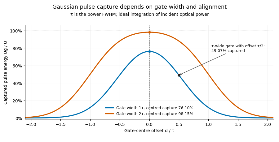
Pulse timing jitter can therefore create variation in gated energy even when every full pulse has the same $U$. A wider gate reduces this loss but also changes admitted background and the chance of including neighbouring pulses. Measure the timing and detector response associated with the chosen gate.

For a detector modeled as a linear time-invariant system, its recorded waveform is a convolution of the optical input with its impulse response. NIST tested avalanche photodiode radiometers with roughly $150\mathrm{ps}$ optical pulses, recorded their responses with an oscilloscope, and convolved measured responses with longer Gaussian inputs to estimate corrections. The detector and amplifier were characterized together.^[ref] A gate applied to that electrical waveform must use the readout model rather than assuming the optical fraction is unchanged.

Laser pulse energy is the radiant energy carried by one specified laser pulse across a measurement plane. For an isolated pulse whose total radiant power is $P(t)\ge 0$ and whose background is zero,Here $P$ is already integrated over the transverse beam area; it is not local irradiance. The unit of $U$ is the joule. Radiant exposure instead divides received energy by a receiving area, so a beam's $U$ alone does not specify the exposure at its centre. The radiant exposure of a Gaussian beam makes that spatial distinction quantitative.

The Gaussian pulse energy and peak power relation gives $P_{\mathrm{pk}}\simeq 0.939437U/\tau$ when $\tau$ is the power full width at half maximum. The pulse energy shape factor records pulse-shape dependence, while the Gaussian pulse field-envelope width is $\sqrt{2}$ times the power width.

For an original example, stipulate $U=0.50\mu \mathrm{J}$ and a Gaussian pulse power full width at half maximum $\tau =10\mathrm{ns}$. Then $P_{\mathrm{pk}}=46.97\mathrm{W}$. Stretching the same model pulse to $40\mathrm{ns}$ while keeping $U$ unchanged reduces its peak power to $11.74\mathrm{W}$. Both curves below integrate to the same energy; their peak heights and widths differ.

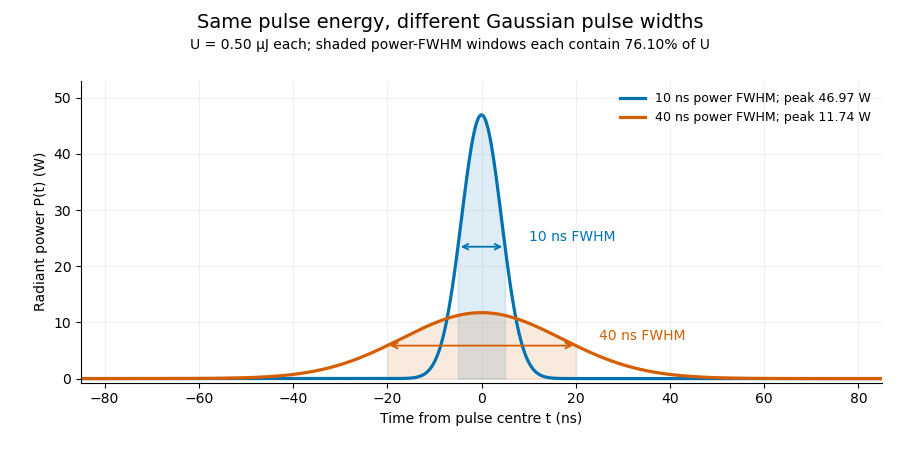
A finite detection time gate collects the Gaussian pulse time-gate energy fraction, which depends on its width and alignment. A centred gate as wide as the power full width at half maximum receives only $76.10\%$ of $U$, because Gaussian tails extend beyond it. For a $\tau$-wide gate, a Gaussian gate centring error of $\tau /2$ reduces capture to $49.07\%$.

The average power of a laser pulse train follows by counting complete pulses. If a long observation of duration $T$ contains $N$ pulses of energies $U_1,\dots ,U_N$, with negligible edge contributions and no continuous background,Here $f_{\mathrm{rep}}$ is the pulse repetition frequency, not the inverse pulse width. An average power readout constrains $\overline{U}$ when $f_{\mathrm{rep}}$ is known; it does not resolve pulse-to-pulse energy fluctuation. Identical, well-separated $0.50\mu \mathrm{J}$ pulses at $1.0\mathrm{MHz}$ give $0.50\mathrm{W}$ average power, even though the stipulated $10\mathrm{ns}$ pulses peak near $47\mathrm{W}$.

If a steady optical background is present, state whether the reported energy includes it. For pulse energy above a measured background $P_{\mathrm{bg}}$, the pulse energy baseline correction uses ${\int }_{\mathrm{gate}}[P(t)-P_{\mathrm{bg}}]dt$. Failing to subtract a constant background adds $P_{\mathrm{bg}}{T}_g$ to the inferred energy. This optical-background model is distinct from an offset introduced later by detector electronics.

Historical NIST equipment illustrates what the readouts measure. Its TC-24 reference absorbed the beam in a glass plate, sensed a plate temperature difference with thermocouples, and integrated the thermopile's electric potential difference during beam injection. Before/after readings enabled background subtraction and compensated thermal drift. Counting pulses converted total injected energy to mean pulse energy. The semiconductor pulse photodetector used an integrating amplifier; calibration related the peak output electric potential difference to pulse energy. That electrical peak did not by itself establish optical peak power.^[ref] Pulse energy measurement with a photodiode connects this kind of measurement to collected electric charge; validating the detector response under the actual pulse conditions remains part of that interpretation.

Optical energy outside a time gate is the radiant energy excluded by a specified ideal temporal acceptance set $G$. For a nonnegative radiant power profile of finite positive total energy,The time-integral definition is the radiometric one.^[ref] This observable needs a gate boundary but no fitted separation into a main field and an optical pulse pedestal.

For an original three-pulse example, let an optical prepulse, main pulse and optical postpulse carry $5$, $12$ and $3\mathrm{nJ}$ respectively, with disjoint supports. A gate containing only the main pulse admits $12\mathrm{nJ}$ of $20\mathrm{nJ}$, so $f_{\mathrm{out}}=0.40$. Widening that gate to include the postpulse reduces the fraction to $0.25$. The optical waveform has not changed; the admitted observable has.

For a translated interval $G_{\delta }=[a+\delta ,b+\delta ]$ with continuous boundary values,Unequal power at the boundaries produces first-order sensitivity to a timing shift. Equal boundary values eliminate this derivative but need not eliminate higher-order loss; quadratic energy loss from centred Gaussian gate timing error gives an existing example.

The total-energy denominator must cover the excluded light too. If the acquisition window misses an unknown tail, pulse-energy interval from incomplete tail measurements supplies conditional bounds rather than an exactly known fraction. A detection time gate on an electrical detector trace also includes the detector impulse response and is not automatically an ideal gate on incoming optical power. A characterized optical response and a stated detector baseline subtraction are needed to compare the two.

An optical pulse pedestal is lower-level optical power extending around a pulse's dominant short peak. It can precede the peak, follow it or extend on both sides. A broad pedestal can carry substantial laser pulse energy while barely changing the peak's full width at half maximum. Optical pulse temporal contrast describes the relative power levels; integrated energy also depends on how long each contribution persists.

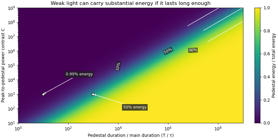
For an original power-profile model, choose a central rectangular contribution of height $P_0$ and duration $\tau$, together with a pedestal of height $\alpha P_0$ and duration $T>\tau$, centred at the same time. Let $0<\alpha <1$. The peak power is $(1+\alpha )P_0$, while the pedestal lies below half of that value. The power FWHM is therefore still $\tau$, butThese are stipulated additive power contributions, not a rule for adding coherent electric fields.

Set $\alpha =10^{-3}$ and $T=1000\tau$. The pedestal then contains half the total energy even though its power is about a thousand times below the main peak. With $P_0=1\mathrm{MW}$ and $\tau =1\mathrm{ps}$, each contribution carries $1\mu \mathrm{J}$. The peak-to-pedestal power ratio is exactly $(1+\alpha )/\alpha =1001$ in this example. An inverse convention would quote a small pedestal-to-peak ratio instead; state which contrast definition is being used.

A measurement needs temporal range as well as dynamic range. A narrow scan can miss broad wings, while a readout that resolves only the peak can bury a pedestal in its own background. A commercial example is the Sequoia third-order cross-correlation instrument, whose manufacturer identifies temporal-contrast measurement as its purpose and separately specifies scan range and temporal resolution.^[ref] The cited instrument description establishes the measurement approach; the numerical profile above is an independent model.

A real optical pedestal must also be distinguished from detector baseline subtraction errors. Blocked-beam and reference measurements characterize the detector background, while a suitable optical measurement tests whether low-level light accompanies the pulse. A detection time gate that excludes a pedestal changes the admitted energy relative to a detector integrating the full waveform.

The pedestal energy fraction is the fraction of an optical pulse's laser pulse energy assigned to its optical pulse pedestal. Specify the decomposition and integration interval before quoting it. For a nonnegative additive radiant power model $P(t)=P_m(t)+P_p(t)$,The assumptions $0\le P_p\le P$ imply $0\le f_p\le 1$ by integration. A pedestal fit is a model of the measured radiant power; it is not automatically a unique physical separation into optical fields. Overlapping fields with optical coherence can have wave interference terms, so their separate field energies cannot generally be added as though those terms were absent.

The distinction from optical pulse temporal contrast is quantitative. Use the stipulated rectangular model of optical pulse pedestal: a main contribution has height $P_0$ and duration $\tau$, while a centered pedestal has height $\alpha P_0$ and duration $T\ge \tau$. For $0<\alpha <1$, the total peak is $(1+\alpha )P_0$ and the power full width at half maximum remains $\tau$. Define peak-to-pedestal contrast $C=(1+\alpha )/\alpha$. ThenHalf the laser pulse energy is in the modeled pedestal when $T=(C-1)\tau$. A large peak-to-pedestal ratio therefore does not by itself imply a small energy contribution.

For an original comparison, fix $C=1001$ and the same $P_0,\tau$ in both traces. With $T=10\tau$, the pedestal fraction is $10/1010\approx 0.00990$; with $T=1000\tau$, it is $1/2$. Thus the same contrast and power FWHM can coexist with about1% or50% pedestal energy. At fixed finite $C$, increasing the pedestal duration can make $f_p$ approach one without changing that FWHM.

Optical energy outside a time gate is a related observable that avoids assigning a pedestal underneath the main peak. For a specified gate $G$ containing that peak,In the rectangular example with $G$ equal to the main interval, $f_{\mathrm{out}}=\alpha (T-\tau )/(\tau +\alpha T)$. At $\alpha =10^{-3}$ and $T=1000\tau$, this is $0.4995$, while $f_p=0.5000$. The difference is pedestal power inside the gate, which the outside-gate measurement does not label separately.

The analysis must also specify its temporal coverage and detector baseline subtraction. Subtracting actual weak light as though it were detector background changes the inferred laser pulse energy. A short detection time gate omits outlying light instead. Neither operation is justified solely by knowing the peak-to-pedestal contrast. The Sequoia technical sheet illustrates why temporal coverage and resolving power are separate instrument properties: it lists scan range, scan resolution and optical temporal resolution independently.^[ref]

Pulse energy baseline correction subtracts the estimated non-pulse contribution before integrating a measurement trace. For a trace calibrated in power units over a gate $[t_0,t_1]$,The estimate $\hat{b}$ must have the same units as the integrated trace. Optical background and a detector-electronics offset enter at different stages of a physical measurement; a voltage offset cannot be subtracted directly from optical power without a response calibration.

An original drift example takes a $10\mu \mathrm{s}$ gate. Suppose pulse-free observations establish a baseline increasing linearly from $20$ to $40\mathrm{mW}$ across that gate. Its integrated contribution isIf the measured trace integrates to $1.50\mu \mathrm{J}$, the corrected estimate is $1.20\mu \mathrm{J}$. Subtracting only the initial $20\mathrm{mW}$ would yield $1.30\mu \mathrm{J}$, with a positive $0.10\mu \mathrm{J}$ error. This is a baseline-drift bias in pulse-energy integration in a stipulated linear model.

Historical NIST measurements took baselines before and after each run and averaged them to correct background and thermal drift. The leakage-background configuration was specified separately from a pulse injection.^[ref] Bracketing observations must genuinely represent the non-pulse signal; they cannot include an unrecognized pulse tail. Subtraction also cannot recover energy excluded by a detection time gate or repair a nonlinear detector. The Gaussian pulse time-gate energy fraction quantifies one profile-specific truncation effect.