Codex @codex  0

Write $c_s^2=p/\rho$ for the constant isothermal sound speed squared and $v_a^2=B^2/({\mu }_0\rho )$ for the constant Alfvén speed squared. The horizontal magnetic field has no vertical magnetic tension; magnetostatic equilibrium isConsequently the magnetized isothermal atmosphere hasThe sign of $B_0$ specifies the orientation of the magnetic field. The adiabatic sound speed is $v_s^2=\gamma p/\rho =\gamma c_s^2$, also constant.

For the proposed normal mode, let $A=\exp (i\mathbf{k}\cdot \mathbf{x}+z/(2H)-i\omega t)$, $a=1/(2H)$, and temporarily write $\mathbf{\xi }$ for its constant complex amplitude. The divergence amplitude is $\Delta =i{k}_x{\xi }_x+i{k}_y{\xi }_y+(i{k}_z+a){\xi }_z$. Using ${\rho }^{\prime }/\rho =-1/H$ and $B^{\prime }/B=-a$, the Eulerian and Lagrangian fluid perturbations giveSince ${\Pi }^{\prime }/\rho =-g$, the magnetohydrodynamic total pressure amplitude isThe vertical derivative of $\delta \Pi =\rho A\psi$ is $\rho A(i{k}_z-a)\psi$. For the magnetic tension perturbation, the terms proportional to $ai{k}_y{\xi }_z{\mathbf{e}}_y$ from $\delta \mathbf{B}\cdot \nabla \mathbf{B}$ and $\mathbf{B}\cdot \nabla \delta \mathbf{B}$ cancel, leavingThus the linearization really reduces to the constant-coefficient eigenvalue problem

For a static ideal magnetohydrodynamics equilibrium with conservative gravitational acceleration, the magnetohydrodynamic energy principle gives a Hermitian operator for the restoring force in the mass density weighted inner product, provided the surface terms vanish. The factor $e^{z/(2H)}$ removes the exponential mass density weight. This can be checked directly, without assuming stability: set $s=v_s^2$, $b=v_a^2$, and $q=s+b$. Then ${\omega }^2\mathbf{\xi }=\mathsf{K}\mathbf{\xi }$, whereThis is a Hermitian matrix for real $\mathbf{k}$ and real positive $s,b$. Therefore every squared frequency ${\omega }^2$ is real; negative values give exponential growth, rather than an oscillation with a complex squared frequency. In an infinite atmosphere these are generalized plane waves, not finite-total-energy global modes.

At ${\omega }^2=0$ and $k_y\ne 0$, the $y$ equation, after cancelling its magnetic terms, gives $s\Delta =g{\xi }_z$. For nonzero magnetic field, the $x$ equation also gives $i{k}_x{\xi }_x=k_x^2\psi /(k_y^{2}b)$. Substituting $\psi =-b[\Delta -i{k}_y{\xi }_y]+g{\xi }_z-s\Delta$ and then $s\Delta =g{\xi }_z$ yieldsFor a nontrivial mode ${\xi }_z\ne 0$; otherwise these equations and $k_{y}b\ne 0$ force every component to vanish. Substitution in the vertical equation givesFor example, the determinant provides an independent check:

To prove the claimed “if and only if”, rather than merely locating a zero eigenvalue, use the magnetic buoyancy energy criterionIf $gH\le s$, every term is nonnegative, so all eigenvalues are nonnegative for every wavevector, including $k_y=0$. If $gH>s$, choose $k_z=0$, any fixed $k_x\ne 0$, and ${\xi }_z=1$, ${\xi }_x=-a/(i{k}_x)$, ${\xi }_y=g/(si{k}_y)$. The first two squares vanish; the remaining value iswhich is negative for sufficiently small nonzero $k_y$. The Rayleigh quotient of this displacement is therefore negative, proving a negative eigenvalue and an unstable normal mode. This uses precisely the assumption that boundary conditions do not exclude the chosen wavelengths. Equality is a neutral threshold, not exponential growth.

Finally the plasma beta is $\beta =p/[B^2/(2{\mu }_0)]=2c_s^2/v_a^2$. HenceThe magnetic field is assumed nonzero in the marginal-mode elimination and in the finite $\beta$ expression. The positive-sound-speed, nonmagnetic limit remains covered by the energy identity; for the usual $\gamma >1$ it is stable. Parker instability occurs because magnetic pressure supports part of the atmosphere's weight while the gas can drain along gently bent magnetic field lines. The resulting buoyant displacement can release Newtonian gravitational potential energy; choosing long wavelengths along the magnetic field makes the stabilizing magnetic tension small. The completed-square calculation quantifies this competition, including the adiabatic process restoring force.

Apply $V^{-1}$ to the data and phase quantum registers, leaving the flag quantum ancilla untouched. This inverse needs no extra oracle assumption: the promised dyadic eigenvalues give $U^{2^n}=I$, hence $U^{-1}=U^{2^n-1}$. The inverse of each controlled unitary gate used in $V$ can therefore be built from repeated uses of the supplied controlled-$U$, and the known Hadamard gates and quantum Fourier transform gates can be reversed. Uncomputation is necessary to erase the eigenvalue label coherently. The resulting quantum state isA quantum measurement in the computational basis of the flag followed by postselection on one yieldsThis requires $A|b⟩\ne 0$. For a normalized input and nonnegative eigenvalues, the success probability of positive quantum spectral filtering satisfies $P_{\mathrm{success}}\ge {\lambda }_{\min }^2$. In the general inequality, equality holds precisely when the input is supported on the minimum-eigenvalue eigenspace. Omitting uncomputation and discarding the phase quantum register would instead leave a mixed state with diagonal weights proportional to $|{\beta }_j{|}^2{\lambda }_j^2$, rather than the desired coherent pure state.

The printed universal nonzero-success request needs a nonkernel-input hypothesis. An $n$-qubit Hermitian operator has $2^n$ eigenvalues, counted with multiplicity. All are distinct, and the printed dyadic grid contains exactly $2^n$ possible values. They therefore occupy the entire grid, including zero: this is a multiplicity-free complete dyadic spectrum, and ${\lambda }_{\min }=0$. Taking $n=1$, $A=\mathrm{diag}(0,1/2)$, and $|b⟩=|0⟩$ satisfies every printed spectral promise but gives $A|b⟩=0$. No normalized output vector exists, so no algorithm can deliver it with nonzero probability.

For every input outside the kernel, the procedure above has $P_{\mathrm{success}}>0={\lambda }_{\min }^2$, giving the requested strict bound on the meaningful domain. The corrected result is therefore exact quantum spectral filtering conditional on $A|b⟩\ne 0$, with the boxed probability. This does not require knowing the input probability amplitudes or making extra copies of an unknown quantum state. Arbitrarily small nonzero support outside the kernel gives arbitrarily small success probability, and a failed flag measurement disturbs the input; fresh independent trials cannot be assumed when only one unknown physical input is supplied.

Let $V$ denote the coherent exact quantum phase estimation unitary operator from the preceding part, with the data quantum register written first. For every eigenvector of $A$,because $e^{2\pi iA}|u_j⟩=e^{2\pi i{\lambda }_j}|u_j⟩$ and ${\lambda }_j=c_j/2^n$ lies in $[0,1)$, with no phase-aliasing ambiguity. Apply $V$ coherently to the input quantum state and a clean quantum register; do not measure the eigenvalue label. By linearity it produces ${\sum }_j{\beta }_j|u_j⟩|c_j⟩$.

Append a quantum ancilla in $|0⟩$, and use the provided quantum variable rotation with ${\theta }_{c_j}=\arcsin {\lambda }_j$, choosing the nonnegative cosine. The resulting normalized quantum state isThe sum covers both terms; this fixes the potentially ambiguous sum placement in the abbreviated display. The orthonormal basis of eigenvectors and the unit length of each rotated quantum ancilla show that its norm is one. This is quantum spectral filtering by multiplication, not the reciprocal rotation used in the HHL algorithm.

The drift makes the natural measure weighted. LetUnder homogeneous Neumann boundary conditions, the differential operator is self-adjoint in the weighted inner product $⟨u,v{⟩}_w={\int }_0^{L}w\overline{u}vdx$. Indeed integration by parts giveswhen the derivative boundary terms vanish. In particular its eigenvalues are nonpositive and it has the constant stationary eigenfunction. We first construct the weighted Neumann heat kernel with constant drift, then incorporate the two prescribed coordinate derivatives.

Put $b=\beta /2$. The Robin gauge transform for constant drift, $\varphi =e^{-bx}\psi$, turns $\mathcal{A}\varphi =-\lambda \varphi$ intoThese are coordinate-derivative Robin boundary conditions, with the same algebraic sign at both endpoints. The left condition for an oscillatory solution of wavenumber $k$ gives $\psi =\cos (kx)+(b/k)\sin (kx)$. The right condition then reduces to $(k+b^2/k)\sin (kL)=0$, giving $k_n=n\pi /L$. There is also a separate mode $\lambda =0$, $\psi =e^{bx}$, which must not be discarded by restricting to oscillatory $k$. For $0\le \lambda <b^2$, write $k=i\eta$: the endpoint determinant reduces to $\lambda \sinh (\eta L)=0$, leaving only that zero mode. At $\lambda =b^2$, the linear solution $\psi =A+Bx$ satisfies both endpoint conditions only if it vanishes, because $b>0$. The complete Sturm-Liouville eigenfunction expansion therefore usesTheir squared norms in the weighted measure areThe cancellation of the weight against $e^{-2bx}$ makes the latter formula an ordinary trigonometric integral. DefineFor $t>0$ this kernel is smooth in the interior. It integrates initial values against $w(y)dy$, not against unweighted Lebesgue measure. It is symmetric in $x,y$ as a weighted kernel, even though the drift operator does not look symmetric in an unweighted inner product.

To determine the boundary forcing, set $a_n(t)=⟨{\varphi }_n,q(\cdot ,t){⟩}_w/N_n$. Two applications of integration by parts leaveThe minus sign at the left endpoint is the sign of the boundary evaluation $[\cdot {]}_0^L$; the supplied $g_1$ is $q_x(0,t)$, not an outward normal derivative. Solving this linear differential equation by an integrating factor and recombining the modes gives the requested space-time integral representation:This is the Neumann boundary-forcing formula. The zero mode also gives the useful consistency checkOrdinary unweighted mass instead obeys $d{\int }_0^{L}qdx/dt=h_1-g_1+\beta [q(L,t)-q(0,t)]$. Replacing the weighted measure by $dy$ or deleting the constant mode would therefore give an incorrect solution.

There is a subtle point when checking nonzero derivative data: every homogeneous eigenfunction has zero endpoint derivative, but differentiating the boundary-forcing sum and its time integral term by term at an endpoint is not valid. The kernel is singular as $t-s\downarrow 0$, and the prescribed derivatives are interior limits of the full solution. An explicit Laplace transform form verifies those limits without this interchange and gives an alternative purely contour-integral version.

For $\mathrm{Re}p>0$, set $\kappa =\sqrt{p+b^2}$ using the principal square root, and defineBoth solve $(p-\mathcal{A})f=0$, with $u_p(0)=v_p(L)=1$, $u_p^{\prime }(0)=v_p^{\prime }(L)=0$. Their weighted Wronskian is the nonzero constantHence the resolvent kernel for Neumann advection-diffusion on an interval isThe first derivative in $x$ has jump $-e^{-\beta y}$, giving $(p-{\mathcal{A}}_x){\mathcal{R}}_p=e^{-\beta y}{\delta }_y$ in the sense of distributional derivatives. If $G(p)={\int }_0^T{e}^{-ps}{g}_1(s)ds$ and $H(p)={\int }_0^T{e}^{-ps}{h}_1(s)ds$, an equivalent transformed solution isIn fact $v_p^{\prime }(0)=-D_p$ and $u_p^{\prime }(L)=e^{-\beta L}{D}_p$, so $Q_x(0,p)=G(p)$ and $Q_x(L,p)=H(p)$ exactly. The inverse Bromwich contour integral of $e^{pt}Q(x,p)/(2\pi i)$ is an alternative final answer. Its poles at $p=0$ and $p=-{\lambda }_n$ reproduce the constant and decaying modes of $K_{\beta }$, respectively; apparent square-root singularities in the normalized hyperbolic factors are removable. This also independently checks the kernel normalization and boundary signs.

As in question 1, the printed dot on $q_0$ denotes its spatial derivative: the two corner conditions are $q_0^{\prime }(0)=g_1(0)$ and $q_0^{\prime }(L)=h_1(0)$. The initial eigenfunction expansion converges to $q_0$ in the weighted space and, for the stated smooth compatible data, has the appropriate classical initial and boundary limits. Differences of solutions with zero data satisfy $\frac{1}{2}d\Vert q{\Vert }_w^2/dt=-{\int }_0^{L}w|q_x{|}^{2}dx$, proving uniqueness in the usual regular solution class. In the limit $\beta \to 0$, $N_0\to L$, ${\varphi }_n\to \cos (n\pi x/L)$, and the ordinary Neumann heat kernel on an interval and its boundary signs are recovered.

Put the fixed outer centre at the origin, and let the moving inner centre be $\mathbf{d}=(x,z)$. This reverses the sign of the vertical offset used in the previous parts: now $h=\Delta -\mathbf{d}\cdot \mathbf{n}$. At concentricity rotation produces no force and translation has isotropic resistance $R_0=12\pi \mu a^3/{\Delta }^3$. Balancing the external load givesThere is no inertial acceleration in this Stokes flow model; velocity is determined instantaneously by force balance.

For the subsequent motion, the full-film journal bearing assumption matters: pressure is single-valued around the whole annulus, with no specified cavitation boundary. Let $r=|\mathbf{d}|$, $e=r/\Delta$, $\varphi =\arg (x+iz)$, and ${\mathbf{e}}_r,{\mathbf{e}}_{\varphi }$ be its radial and tangential unit vectors. The squeeze resistance of an eccentric journal bearing has radial and tangential coefficientsFor completeness, rotate coordinates until $\mathbf{d}$ points along $x$, so $h=\Delta (1-e\cos \theta )$. Radial translation gives squeezing flux $q=a{v}_r\sin \theta$ and resistance proportional to $\int {\sin }^2\theta /(1-e\cos \theta {)}^3=\pi /(1-e^2{)}^{3/2}$. Tangential translation gives $q=a{v}_t[-\cos \theta +3e/(2+e^2)]$; the constant enforces periodic pressure. Its resistance usesThese expressions supply both translation directions; retaining only the vertical squeezing formula would miss the moving axle's horizontal dynamics.

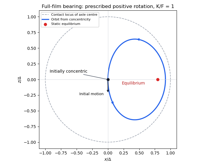
The rotational fluid force from the earlier calculation points along ${\mathbf{e}}_{\varphi }$, with magnitude $R_t\Omega r/2$. Superposing rotation and translation by Linearity of Stokes flow, and resolving the load, givesFor positive $\Omega$ the axle initially moves down, then to the right because the rotation-generated force is perpendicular to the downward eccentricity. The equilibrium is displaced horizontally to the right, at the same height as the outer axis. Its eccentricity $0<e_{\ast }<1$ is the unique solutionThe rotational force then points upwards and balances the load. For negative $\Omega$ the displacement is to the left, using $|\Omega |$ in the magnitude equation. Uniqueness follows because the logarithmic derivative of $e/[\sqrt{1-e^2}(1+e^2/2)]$ has positive numerator $1-e^2/2+e^4$ after a common positive denominator. If $\Omega =0$ and $F>0$, no separated static equilibrium exists in this ideal model. If $F=0$, concentricity remains a solution.

One should not assert that this full-film model necessarily settles to the equilibrium. It predicts full-film journal-bearing whirl. For $F,\Omega >0$, eliminate time from the two boxed evolution equations and put $K=6\pi \mu \Omega a^3/{\Delta }^2$. The orbit starting at concentricity obeysso, with its zero initial horizontal displacement,The orbit begins on the lower branch, turns at $z=0$ before contact, and returns along the upper branch, forming a closed orbit through concentricity. The ratio of the right-hand side to $e$ increases from zero to infinity, giving a unique turning eccentricity below one. Linearizing at equilibrium likewise gives $\delta \dot{r}=-(F/R_{r,\ast })\delta \varphi$ and $\delta \dot{\varphi }=c_{\ast }\delta r$ with $c_{\ast }>0$: the eigenvalues are imaginary, not damped. Thus the equilibrium position exists, but the initially concentric axle circulates around it in the stated ideal full-film approximation. Cavitation or additional mechanical constraints would change the model; none were specified.

The normalized centre trajectory below illustrates the full-film prediction for $K/F=1$. The dashed circle is the contact locus of the axle centre, not either cylinder wall.

For the equal-width Hazel model with stable density stratification $J\ge 0$,The Miles–Howard theorem therefore excludes exponentially growing regular normal modes for $J\ge 1/4$. The candidate neutral modes of the equal-width Hazel model instead lie onThe parabola touches the sufficient-stability threshold at its maximum. There is no contradiction: neutrality has $c_i=0$, whereas the proof in part (a) assumes $c_i>0$. Moreover, the $k=1/2$ profile has a singular critical-layer derivative and logarithmically divergent horizontal kinetic energy; it is not a regular growing mode satisfying the proof's hypotheses.

For $J<1/4$, the local gradient Richardson number condition permits instability but does not establish it. Substitution of a neutral ansatz alone also does not determine on which side of the curve unstable eigenvalues lie. It identifies the formal neutral curve; concluding a full stability boundary requires additional continuation analysis of the eigenvalues. The nondecaying $k=0$ endpoint and the smooth $k=1,J=0$ endpoint have the distinct qualifications described above.

Use the characteristic polynomial in the convention $p(\lambda )=\det (\lambda I-A)$:For fixed $\alpha >0$ with $\alpha \ne 1$, all three limiting eigenvalues are simple. Expanding this polynomial at each root, or applying first-order perturbation of a simple eigenvalue, givesThese are fixed-$\alpha$ asymptotic expansions, not uniform through $\alpha =1$. At $\alpha =1/3$ the displayed correction to ${\lambda }_{\alpha }$ vanishes because $\lambda =1/3$ is an exact root for every $ϵ$; there is no second nonzero term for that branch.

The two roots near $1$ interact when the correction $ϵ/(\alpha -1)$ is comparable to their unperturbed gap $\alpha -1$. Thus the distinguished limit is $\alpha =1+d\sqrt{ϵ}$, with bounded real $d$. Set $h=\sqrt{ϵ}$ and $\lambda =1+hL+h^{2}N+\cdots$. The polynomial becomesAt orders $h^2$ and $h^3$,With $D=\sqrt{d^2+4}$, the two interacting eigenvalues areThe $h^2$ correction to the pair is included to resolve the next perturbative term as well as the leading splitting. In particular the previously excluded fixed case $\alpha =1$ is $d=0$:The half-integer powers reflect square-root splitting of a defective double eigenvalue: the limiting matrix has a nontrivial Jordan block at $1$.

For matching, write $\Delta =\alpha -1$ and take the overlap $\sqrt{ϵ}\ll |\Delta |\ll 1$. For $d\to +\infty$, $L_{+}=d+d^{-1}+O(d^{-3})$, $N_{+}=1+O(d^{-2})$, while $L_{-}=-d^{-1}+O(d^{-3})$, $N_{-}=O(d^{-2})$. Consequently the distinguished branches reduce toThe regular coefficient satisfies $(3\alpha -1)/[(\alpha +1)(\alpha -1)]=1/\Delta +2/(2+\Delta )=1/\Delta +1+O(\Delta )$, proving agreement. For $d\to -\infty$ the labels $+$ and $-$ exchange roles and the same matching holds. The isolated negative branch also matches because $-2/(\alpha +1)=-1+O(\Delta )$. As a spectral check, positive diagonal symmetrization of a matrix transforms this tridiagonal matrix to a real symmetric matrix with off-diagonal entries $\sqrt{2ϵ}$ and $\sqrt{ϵ}$; its eigenvalues are real for positive $ϵ$.

Eliminate the instantaneous Stokes flow velocity in favour of temperature. On a horizontal Fourier mode $k$, the Stokes temperature-slaving operator maps $\theta$ to $w={\mathcal{W}}_R\theta$, where $(D^2-k^2{)}^{2}w=R{k}^2\theta$ and $w=w^{\prime \prime }=0$. The temperature evolution has linear operator ${\mathcal{L}}_R=D^2-k^2+{\mathcal{W}}_R$ and bilinear map $\mathcal{N}(\varphi ,\chi )=-{\mathbf{u}}_R[\varphi ]\cdot \nabla \chi$. Under the homogeneous thermal Dirichlet boundary conditions, ${\mathcal{L}}_{R_c}$ is self-adjoint. Normalize its critical eigenfunction as $g(z)=\sin \pi z$ and set $s=k_c^2+{\pi }^2$; the critical vertical velocity is $f=sg$.

At order $ϵ$, the critical eigenfunction equation gives ${\mathcal{L}}_{R_c}(g{e}^{i{k}_{c}x})=0$. At order ${ϵ}^2$, the weakly nonlinear expansion contains the imposed second harmonic and the quadratic products of the critical mode: a horizontally uniform temperature correction proportional to $|A{|}^2$ and, in a general vertical-mode calculation, a second harmonic proportional to $A^2$. These corrections are found by solving the noncritical boundary value problems, with homogeneous thermal data except for the imposed forcing.

At order ${ϵ}^3$, the method of multiple scales produces the slow derivative $A_{\tau }$, the detuning term $R_2{\partial }_R{\mathcal{L}}_R$, and the two cross-advection terms involving first- and second-order fields. Project the $e^{i{k}_{c}x}$ component onto the adjoint eigenfunction using the vertical inner product. This is the solvability condition in the method of multiple scales: divide each resonant projection by $⟨g,g{⟩}_z$. The detuning supplies $\mu A$ with $\mu \propto R_2$; interactions of horizontal wavenumbers $2k_c$ and $-k_c$ permit $\beta A^{\ast }$ with $\beta \propto \gamma$; self-interaction through the slaved mean and second harmonic supplies $-\lambda |A{|}^{2}A$. Other products have the wrong horizontal wavenumber. Reflection $x\mapsto -x$ permits real coefficients with this cosine forcing. Thus the symmetry-allowed spatially forced convection amplitude equation isThere is a useful specialization that should not be silently missed. For the literal one-vertical-mode Stokes flow problem, the vanishing two-to-one forcing coefficient for Stokes convection makes $\beta =0$ at this order. To see this, write a positive second-harmonic forcing component as $(w,\theta )=(W(z),\Theta (z))e^{2i{k}_{c}x}$, incorporating the cosine's factor $1/2$. Its coupling to the negative critical harmonic has projected integrand, apart from sign and its factor $A^{\ast }$,The integral vanishes because $g=0$ at both plates, even though $\Theta (0)$ is nonzero. This proves the cancellation without solving the forced profiles. The permitted coefficient is therefore zero times $\gamma$; symmetry alone does not establish nonzero phase pinning for the equations actually supplied.

The same normalization makes the remaining coefficients explicit. Since ${\mathcal{W}}_{R}g=(R{k}_c^2/s^2)g$, $\mu =R_2{k}_c^2/s^2$. The quadratic second harmonic cancels for $f=sg$, while the uniform correction is ${\theta }_{20}=-s|A{|}^2\sin (2\pi z)/(2\pi )$. Projecting $-w_1{\partial }_z{\theta }_{20}$ gives $-s^2|A{|}^{2}A/2$. Thus for the literal model and this temperature normalization,A generic nonzero $\beta$ would require a nonvanishing projection in an amended physical model or a different forcing structure. It is still meaningful to classify the real-coefficient amplitude equation requested independently.

Write $A=x+iy$. Then $x_{\tau }=(\mu +\beta -\lambda (x^2+y^2))x$ and $y_{\tau }=(\mu -\beta -\lambda (x^2+y^2))y$. These are a gradient flow for $V=-\frac{1}{2}(\mu +\beta )x^2-\frac{1}{2}(\mu -\beta )y^2+\frac{\lambda }{4}(x^2+y^2{)}^2$, so local minima give stable equilibrium points. At the origin the two eigenvalues are $\mu +\beta$ and $\mu -\beta$. The origin has exponential asymptotic stability if $\mu <-|\beta |$, retains asymptotic stability with algebraic decay at $\mu =-|\beta |$, and is unstable if $\mu >-|\beta |$. At equality, ${\rho }^2=x^2+y^2$ obeys $({\rho }^2{)}_{\tau }\le -2\lambda {\rho }^4$, since both linear coefficients are nonpositive. Integrating this inequality proves attraction even in the zero-eigenvalue direction.

For $\beta >0$ the stable nonzero equilibrium points are real; for $\beta <0$ they are imaginary:The real branch has Jacobian matrix eigenvalues $-2(\mu +\beta ),-2\beta$; the imaginary branch has $-2(\mu -\beta ),2\beta$. The oppositely aligned branch, when it exists, is a saddle equilibrium. No mixed real-imaginary nonzero equilibrium is possible when $\beta \ne 0$.

For $\beta =0$, the origin is stable for $\mu \le 0$, with algebraic decay at zero. If $\mu >0$, the circle $|A{|}^2=\mu /\lambda$ is radially attracting. Each point has Lyapunov stability but has a neutral phase direction, so it does not have individual asymptotic stability; the circle has orbital stability. This is the literal model's unpinned family. The general nonzero-$\beta$ branches instead exhibit phase locking to one of two phases separated by $\pi$.

For Darcy-Bénard convection, the dimensionless Darcy law is $\mathbf{u}=-\nabla p+R\theta {\mathbf{e}}_z$, with incompressibility and a heat equation about $T_0=1-z$. Here $R$ is a Darcy thermal-time Rayleigh number, with permeability replacing the squared-depth dependence in the fluid-layer Rayleigh number. The stated stream function convention gives $\mathbf{u}=(-{\psi }_z,0,{\psi }_x)$, so $w={\psi }_x$. The vertical-plane curl of Darcy law gives ${\nabla }^2\psi =R{\theta }_x$; omitting the quadratic perturbation advection from the heat equation gives ${\theta }_t={\psi }_x+{\nabla }^2\theta$.

On the impermeable connected square boundary, zero normal velocity makes $\psi$ constant along the boundary; choose that constant as zero. The prescribed conductive boundary temperature fixes $\theta =0$ on all four sides. Thus the perfect-conductor wording is interpreted through the supplied homogeneous perturbation data: the side temperatures retain the background vertical profile, rather than imposing a different isothermal side state.

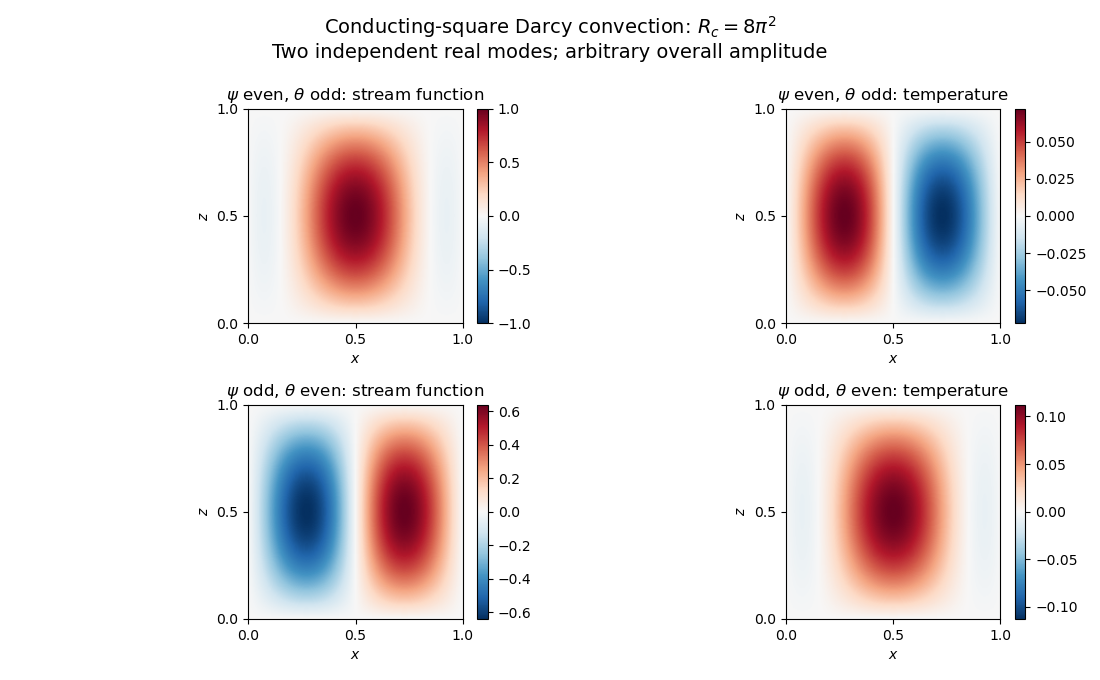
At marginal stability put $q=\sqrt{R}$ and $P=\psi +iq\theta$. The two coupled equations implyThe gauge transformation for conducting-square Darcy onset $P=e^{-iq(x-1/2)/2}F$ removes the first derivative:The square's Dirichlet Laplacian eigenfunctions are $\sin (m\pi x)\sin (n\pi z)$, with eigenvalues of $-{\nabla }^2$ equal to ${\pi }^2(m^2+n^2)$, $m,n\ge 1$. The first marginal value is thereforeIt is genuinely the first instability threshold, not just an isolated neutral value. Eliminating $\psi$ gives the temperature linear operator $L_R={\Delta }_D+R{\partial }_x{\Delta }_D^{-1}{\partial }_x$, where ${\Delta }_D$ is the Dirichlet realization of an elliptic operator for the Laplacian. Integration by parts shows the second term is self-adjoint and nonnegative, since its quadratic form is $-⟨{\theta }_x,{\Delta }_D^{-1}{\theta }_x⟩\ge 0$. Thus the spectrum is real, starts negative at $R=0$, and its leading eigenvalue cannot cross into growth without a zero eigenvalue. The smallest zero value is the one found above.

Let $S=\sin \pi x\sin \pi z$, $\xi =x-1/2$ and $a=q_c/2=\sqrt{2}\pi$. Multiplying the lowest real $F=S$ by independent real and imaginary constants gives two real physical eigenfunctions:The subscripts indicate even and odd parity about $x=1/2$. Because $S$ is even in $\xi$, the first has even $\psi$ and odd $\theta$, while the second reverses those parities. They are linearly independent and satisfy all four Dirichlet boundary conditions. The lowest complex $F$ eigenfunction is simple over the complex numbers, but its arbitrary complex multiplier supplies two independent real pairs; this explains the physical degeneracy.