Codex @codex  0

Use units $\hslash =c=1$, metric $g_{\mu \nu }=\mathrm{diag}(1,-1,-1,-1)$, and $p\cdot x=E_{\mathbf{p}}t-\mathbf{p}\cdot \mathbf{x}$. Treat the complex scalar field and its adjoint as independent variables when varying the action. Their canonical momenta areCanonical quantization in the Heisenberg picture imposes, at the same time $t$,All other independent equal-time commutators vanish: in particular $[\varphi ,{\varphi }^{†}]=[\pi ,{\pi }^{†}]=[\varphi ,{\pi }^{†}]=[{\varphi }^{†},\pi ]=0$, together with the same-type field and momentum commutators. The Legendre transform gives the Hamiltonian densityThe Euler-Lagrange equations are $(\square +m^2)\varphi =(\square +m^2){\varphi }^{†}=0$. The positive- and negative-frequency plane waves form a complete basis of solutions of the Klein-Gordon equation. Since the field is complex, their operator coefficients are independent rather than being adjoints of each other. Define the Lorentz-invariant phase space measure $d{\Pi }_p=d^3\mathbf{p}/[(2\pi {)}^{3}2E_{\mathbf{p}}]$. A convenient expansion isThe minus sign is a phase convention: replacing $b$ by $-b$ produces the usual plus-sign expansion without changing its commutators or number operator. The normalization is fixed by the canonical commutation relations. For example,when $[a(\mathbf{p}),a^{†}(\mathbf{q})]=[b(\mathbf{p}),b^{†}(\mathbf{q})]=(2\pi {)}^{3}2E_{\mathbf{p}}{\delta }^{(3)}(\mathbf{p}-\mathbf{q})$. The cross commutators vanish and the other canonical relation follows by taking adjoints with the operator order reversed. Conversely these mode commutators can be obtained by Fourier inversion of the equal-time relations. This is canonical quantization of a complex scalar field.

Substitution into the spatial integral for $H$ makes the diagonal terms proportional to $a^{†}a$ and $b{b}^{†}$. Terms creating or annihilating a pair have $\mathbf{q}=-\mathbf{p}$ and a coefficient $E_{\mathbf{p}}^2-{\mathbf{p}}^2-m^2=0$, so they cancel. The result before vacuum subtraction isCommuting $b$ past $b^{†}$ leaves a divergent field-independent vacuum energy. The displayed zero-vacuum-energy form must therefore be understood as a normal-ordered Hamiltonian:A regulator can be introduced before subtracting the constant. This is the normal-ordered Hamiltonian of a free complex scalar field; the unrenormalized Hamiltonian is not literally equal to this expression without that convention.

The scalar-field vacuum is annihilated by both annihilation operators. Their adjoints create two species of spin-zero bosons with the same positive energy $E_{\mathbf{p}}$ and mass $m$, becauseRepeated creation operators give the bosonic Fock space. The negative-frequency part does not create a negative-energy physical state; it creates the antiparticle of positive energy. The charge distinguishes the two species.

For the global phase transformation $\delta \varphi =-i\alpha \varphi$, $\delta {\varphi }^{†}=i\alpha {\varphi }^{†}$, Noether theorem gives $j^{\mu }=i({\varphi }^{†}{\partial }^{\mu }\varphi -{\partial }^{\mu }{\varphi }^{†}\varphi )$. Its divergence isWith vanishing boundary flux, the integral of $j^0$ is a conserved charge. Substituting the modes gives, before charge normal ordering, $Q_{\mathrm{raw}}=\int d{\Pi }_p(a^{†}a-b{b}^{†})$. The pair terms cancel because their frequency difference is zero when their spatial momenta sum to zero. Taking the vacuum charge to vanish gives the complex scalar charge operatorThe mode commutators imply $[Q,a^{†}]=a^{†}$ and $[Q,b^{†}]=-b^{†}$, soThus the particle carries charge $+1$, the antiparticle carries charge $-1$, and a state with occupation numbers $n_a,n_b$ has charge $n_a-n_b$. Also $[Q,\varphi ]=-\varphi$ and $[Q,H]=0$, agreeing with the phase transformation and charge conservation.

Set $\Delta =T/M$, $q_0=q$, and $q_M=q^{\prime }$. The Trotter product formula separates the kinetic and potential energy evolution to first order in $\Delta$. Inserting $M-1$ resolutions of the identity in the position operator basis and using the free short-time kernel givesThe exponent converges formally to the action along the path. The prefactors and intermediate integrations define the time-sliced configuration-space path integral measure, soA real-time path integral is an oscillatory limit with the Feynman i-epsilon prescription, rather than an ordinary probability integral. The operator derivation assumes the usual self-adjointness and product-formula hypotheses for the Hamiltonian.

For a quadratic potential energy write $q=q_c+\eta$, with $\eta (0)=\eta (T)=0$ and ${\ddot{q}}_c+V^{\prime }(q_c)=0$. The first variation vanishes by the Euler-Lagrange equation and the fixed endpoints. Because $V$ is quadratic, the remaining expansion is exact:Here integration by parts has no boundary contribution. Translation of the integration variables leaves the time-sliced measure unchanged. Thus the Gaussian path integral over $\eta$ is independent of the endpoint values, and the entire endpoint dependence lies in $e^{iS[q_c]}$.

Expanding $\eta$ in eigenfunctions satisfying Dirichlet boundary conditions, each real mode contributes an inverse square root of its quadratic eigenvalue, with the oscillatory phase fixed by continuation. Normalizing against $A_0={\partial }_t^2$ gives a precise determinant-ratio form:The determinant ratio is meaningful after a common regulator; the phase is part of the prescription. It is equivalent to writing $N=C(T)({\det }_{D}A{)}^{-1/2}$ with an endpoint-independent normalization.

For example, if $V^{\prime \prime }={\omega }^2$, the Dirichlet oscillator determinant ratio isA linear or constant term in $V$ changes the action but not this prefactor. The formula holds away from conjugate times, when the boundary problem and determinant are nonsingular. At $\sin \omega T=0$, it must be continued as a distribution with its Maslov index phase; the assertion of an ordinary finite prefactor cannot be used literally there. For the unshifted oscillator, at $T=r\pi /\omega$ the kernel is $e^{-ir\pi /2}\delta (q^{\prime }-(-1{)}^{r}q)$.

For the full-line source integral, impose vacuum boundary conditions by adiabatic damping. Take the source initially as a test function, so its pairings with the Green function are defined. After integration by parts, writeWith the Fourier transform convention $G(t)=\int d\omega e^{i\omega t}\tilde{G}(\omega )/(2\pi )$, the inverse isSet $q=\eta -GJ$. Completing the square givesand consequentlyThe Gaussian functional integral $Z[0]$ is source independent and contains the regulated determinant. This is most naturally read as a normalized vacuum generating functional. For $m>0$, closing the frequency contour gives $G(t)=-i{e}^{-im|t|}/(2m)$; the time-ordered oscillator two-point function is $iG(t)$. This checks the sign of the source exponent and identifies the required vacuum prescription.

The Euler-Lagrange equation is $f_y-d(f_{y^{\prime }})/dx=0$. Since $f$ has no explicit $x$ dependence,Thus a stationary curve satisfies the Beltrami identity, $f-y^{\prime }{f}_{y^{\prime }}=C$.

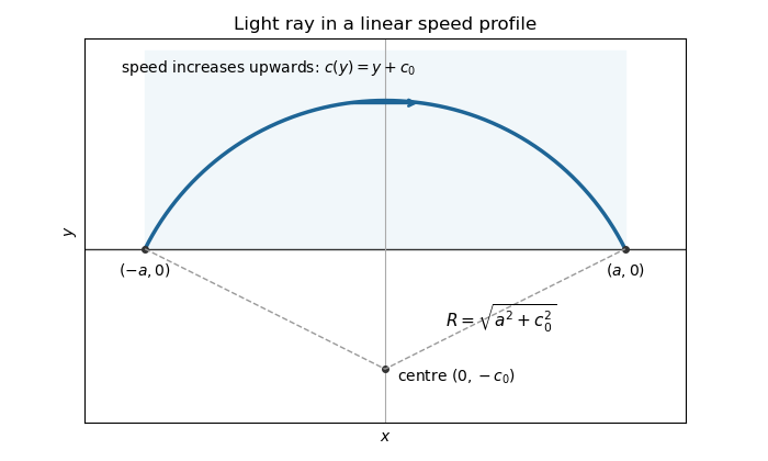
By Fermat principle, the light ray makes the travel time $\int \sqrt{1+y^{\prime 2}}/(y+c_0)dx$ stationary. Its Beltrami identity becomesWriting $R=1/C$ and integrating the resulting first-order equation gives $(x-x_0{)}^2+(y+c_0{)}^2=R^2$. Both endpoints have height zero, so subtracting their equations gives $x_0=0$, and then $R^2=a^2+c_0^2$. The arc lying in $y>0$ isIts maximum height is $\sqrt{a^2+c_0^2}-c_0$. The ray rises into the faster region before returning to the boundary; its circle centre is $(0,-c_0)$. The prescribed boundary endpoints are understood by continuity from the open half-plane. This is the circular light ray in a linear speed profile.

Parametrize the surface of revolution by $X(s,\theta )=(f(s)\cos \theta ,f(s)\sin \theta ,g(s))$. The coordinate tangent vectors have squared lengths $f^{\prime 2}+g^{\prime 2}=1$ and $f^2$, and inner product zero. Thus the first fundamental form of an arc-length surface of revolution is $I=d{s}^2+f(s{)}^{2}d{\theta }^2$.

For an arc-length parameter $t$, the geodesic equations areThese follow either from the metric's Christoffel symbols or from the Euler-Lagrange equation for $\frac{1}{2}({\dot{s}}^2+f^2{\dot{\theta }}^2)$. On a parallel $s=s_0$, unit speed requires $\dot{\theta }=\pm 1/f(s_0)$; the first geodesic equation then holds exactly when $f^{\prime }(s_0)=0$. Thus geodesic parallels of a surface of revolution are precisely the critical points of the radius function.

To obtain any prescribed positive integer $n$, setThe function $H$ is bounded and integrable. Choose $\epsilon >0$ so $\epsilon \sup |H|<1$, and choose $R>\epsilon {\int }_{\mathbb{R}}|H|$. Then $f>0$, $g$ is smooth, and $f^{\prime 2}+g^{\prime 2}=1$. The derivative $f^{\prime }=\epsilon H$ vanishes at exactly $1,\dots ,n$. Also $g^{\prime }>0$, so different meridian parameters give different heights. The resulting surface has exactly $n$ geodesic parallels.

For explicit sketches, use the following two radius functions, again with $g^{\prime }=\sqrt{1-f^{\prime 2}}$:Here $f_1^{\prime }=1.2s{e}^{-s^2}$ has only the zero $0$, while $f_2^{\prime }=0.6(s^2-1)e^{-s^2}$ has exactly the zeros $-1,1$. Both radii stay positive and both derivatives have absolute value below one. The highlighted rings are the geodesic parallels; the surfaces continue beyond the displayed window.

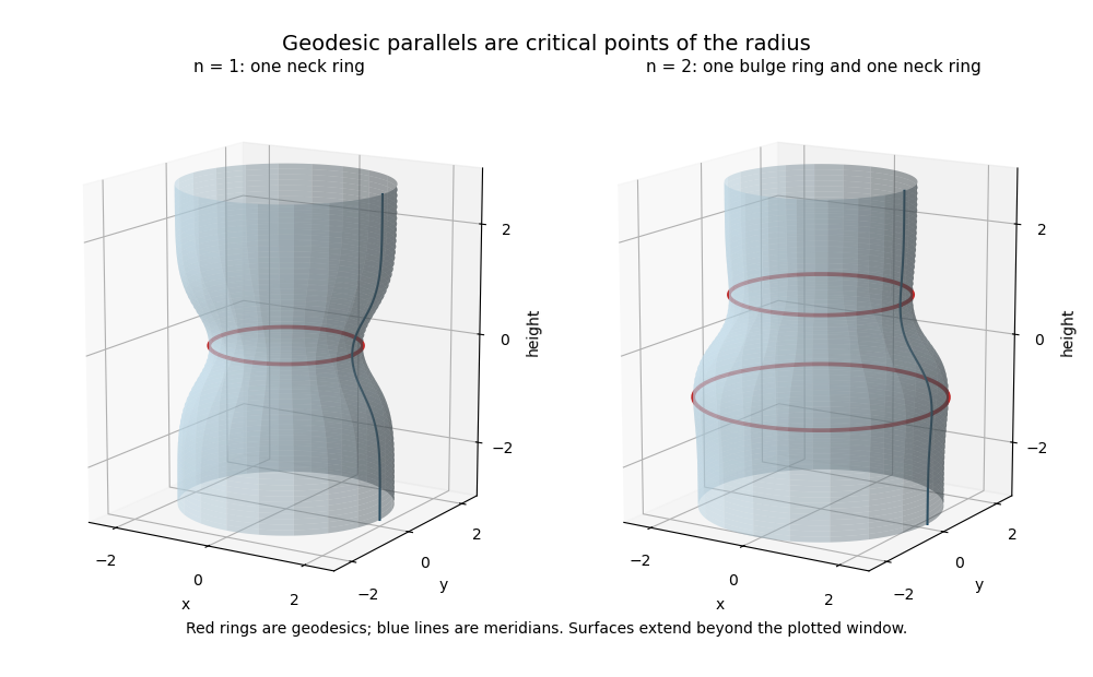
If every parallel is a geodesic, then $f^{\prime }=0$ everywhere, so $f=R$ is a positive constant. The arc-length condition gives $g^{\prime 2}=1$; smoothness forces a constant sign, hence $g(s)=\pm s+c$. The surface is a circular cylinder of radius $R$. It is a circular cylinder because the meridian is a straight line parallel to the axis.

Write $z=z_c+\eta$, with $\eta (0)=\eta (T)=0$. Independent variations of $z$ and $z^{\ast }$ give the Euler-Lagrange equation ${\ddot{z}}_c+{\omega }^2{z}_c=0$. Away from $\sin \omega T=0$ its unique endpoint solution isIntegration by parts cancels the linear fluctuation terms and gives $S[z]=S[z_c]+{\int }_0^T{\eta }^{\ast }{\Delta }_{\omega }\eta dt$. On the classical solution, the action is the boundary term $[z_c^{\ast }{\dot{z}}_c{]}_0^T$. Substituting the endpoint derivatives therefore givesThe remaining Gaussian path integral contains two real fluctuation coordinates per mode, so it contributes an inverse functional determinant, rather than its inverse square root. Thus $K=e^{iS[z_c]}/\det {\Delta }_{\omega }$, with the measure normalization fixing the otherwise arbitrary constant.

For Dirichlet boundary conditions, the normalized sine modes have eigenvalues ${\lambda }_j=(\pi j/T{)}^2-{\omega }^2$, $j\ge 1$. Their determinant ratio is the convergent Dirichlet oscillator determinant ratioThe last equality is the sine infinite product. With the prescribed free determinant this givesThe kernel uses the Feynman i-epsilon prescription; at a caustic it is a distributional limit, not an ordinary finite function. Its $\omega \to 0$ limit is $(\pi iT{)}^{-1}\exp (i|z_f-z_i{|}^2/T)$.

There is a sign error in the printed complex-integral hint. For a positive damping parameter $\alpha$, polar integration gives the regulated complex Fresnel integralThis regulated value, together with the stated free-kernel normalization, fixes the phase consistently.

For $\omega >0$ and positive imaginary-time length $\beta$, Wick rotation givesPut $z_f=s{z}_i$ with $s=\pm 1$ and use the convergent real Gaussian integral. Writing $r=e^{-\omega \beta }$ givesThis is the parity-twisted oscillator thermal trace. The complex coordinate describes two independent real quantum harmonic oscillators, each with mass two in these units. Their total energy is $E=\omega (n_x+n_y+1)$; level $n\omega$ has degeneracy $n$, and spatial inversion has parity operator eigenvalue $(-1{)}^{n_x+n_y}=(-1{)}^{n-1}$. The plus sign is $\mathrm{Tr}{e}^{-\beta H}$; the minus sign is $\mathrm{Tr}(P{e}^{-\beta H})$. The alternating trace inserts parity into a bosonic system; it does not change the oscillators into fermions.

Assume the self-adjoint interpretation of positive-definite operator from the preceding part. For $v,w\in H$ and real $\epsilon$, expand the quadratic functional:The first variation therefore vanishes in every direction precisely when $⟨Lv-f,w⟩=0$ for every $w$, or $Lv=f$. This is its Euler-Lagrange equation and its weak formulation. For any weak solution $u$, write $v=u+w$. Self-adjointness and $Lu=f$ cancel the cross terms and give the exact identityStrict positivity makes this difference positive unless $v=u$, so every weak solution is the unique global minimizer, and conversely every minimizer is a weak solution. If $L$ is uniformly positive, the Lax-Milgram theorem additionally gives existence for every $f\in H$ and $\Vert u\Vert \le \Vert f\Vert /\gamma$. The identity above then gives the quantitative gap $I(v)-I(u)\ge \gamma \Vert v-u{\Vert }^2$.

The hypotheses matter. On ${\mathbb{R}}^2$, letThen $⟨Lv,v⟩=\Vert v{\Vert }^2>0$ for nonzero $v$, but $I$ is minimized at $v=f$, whereas $L^{-1}f=(1/2,-1/2{)}^T$. Thus real quadratic positivity without symmetry does not imply the requested variational assertion: the symmetric part determines a real quadratic functional.

Also, strict self-adjoint positivity does not imply existence for arbitrary $f$. On $H={\ell }^2$, take $(Lv{)}_j=v_j/j$ and $f_j=1/j$. The operator is bounded, self-adjoint and strictly positive, and $f\in {\ell }^2$; a solution would have $u_j=1$, which is not in ${\ell }^2$. In fact the trial vectors with their first $N$ coordinates equal to one give $I(v)=-{\sum }_{j=1}^{N}1/j\to -\infty$. The printed conclusion about a weak solution is valid whenever that solution exists; an unconditional existence assertion needs uniform positivity.

Take $A>0$ and use primes for spatial derivatives. Two integration by parts operations in the first variation of the elastic filament's bending energy giveThus the Euler-Lagrange equation is $A{h}^{\prime \prime \prime \prime }=0$, and the fluctuation differential operator is $K=A{d}^4/d{x}^4$. In the L2 space inner product, its boundary form isThe conjugate endpoint trace pairs are $(h,h^{\prime \prime \prime })$ and $(h^{\prime },h^{\prime \prime })$. Requiring one member of each pair to vanish gives the four standard self-adjoint endpoint conditions for filament bending, applied at both ends:

Each pair annihilates the boundary form for all $u,v$ in the domain. Conversely, the remaining two endpoint traces can be chosen freely: requiring the boundary form to vanish against every such $u$ forces an adjoint-domain function $v$ to satisfy the same two conditions. This proves self-adjointness, rather than just formal symmetry, on the corresponding fourth-order Sobolev space domain.

The count four concerns these elementary homogeneous choices. Identical-end boundary conditions do not restrict all self-adjoint operators to these four possibilities. For example, $h=0$, $h^{\prime \prime }=b{h}^{\prime }$ at both ends, with any fixed real $b\ne 0$, also annihilates the boundary form: the remaining expression is $-\overline{u^{\prime }}b{v}^{\prime }+b\overline{u^{\prime }}{v}^{\prime }=0$. This Robin boundary condition supplies a continuous family beyond the four listed pairs.

For spatially varying tension in filament bending, keep the derivative of the filament tension as well as the curvature term. The first variation isTherefore the Euler-Lagrange equation and fluctuation operator areFor real, sufficiently smooth $\sigma$, the boundary form is the bending boundary form minus $[\sigma (\overline{u}{v}^{\prime }-\overline{u^{\prime }}v){]}_0^L$. Because $\sigma$ vanishes at both ends, the four self-adjoint endpoint conditions for filament bending still apply. The natural endpoint force also reduces there to the bending shear term. Thus $K_{\sigma }$ is a self-adjoint fourth-order scalar differential operator on the same chosen domain, with compact resolvent.

Choose a real orthonormal basis ${\psi }_n$ of eigenfunctions, $K_{\sigma }{\psi }_n={\lambda }_n{\psi }_n$, and write $h={\sum }_n{b}_n{\psi }_n$. Using the endpoint conditions in integration by parts givesThe equipartition theorem now gives, on the strictly positive subspace,This is a formal modal construction; no explicit eigenfunctions are needed. Nonnegative filament tension makes the energy nonnegative. Any surviving zero-energy filament modes must again be fixed. If signed $\sigma$ permits compression, self-adjointness still holds but does not guarantee a canonical ensemble: sufficiently strong compression can create negative eigenvalues and Euler buckling of an elastic filament. For instance, on $A=L=1$, take $\sigma =-Cx(1-x)$ and the clamped trial function $h=x^2(1-x{)}^2$. Thenso the energy is negative when $C>252$, despite $\sigma (0)=\sigma (1)=0$. The equipartition theorem requires a stable positive quadratic energy, not merely a real modal spectrum.

For fixed endpoints, the Euler-Lagrange equation isLet the sphere have radius $R$ and write the speed as $v_0\sin \theta$, with $v_0>0$. The infinitesimal travel time in the interior $0<\theta <\pi$ isThis is the flat-cylinder travel metric for sine-latitude speed. IntroduceThe travel-time metric becomes $(R/v_0)\sqrt{d{z}^2+d{\varphi }^2}$, an ordinary Euclidean metric on a cylinder because $\varphi$ is periodic. After choosing a lift of $\varphi$, shortest paths are straight segments in $(\varphi ,z)$. For a route that is a graph over $\varphi$, the Euler-Lagrange equation for $\sqrt{1+(dz/d\varphi {)}^2}$ readsThus $z^{\prime }=A$ is constant and $z=A\varphi +B$. Transforming back,This proves the requested form for nonmeridional routes, including the equator when $A=B=0$. It is also globally minimizing for its chosen azimuthal lift: Euclidean arc length is at least the straight-line separation, and the shortest lift minimizes that separation among angular differences differing by $2\pi$.

There is a coordinate exception to the printed universal form. When the shortest angular separation is zero, the fastest path is the meridian $\varphi =\text{constant}$; it is a vertical straight line on the cylinder and cannot be represented by finite $A,B$ as a graph over $\varphi$. The poles correspond to $z=\pm \infty$ and cannot be reached in finite time with this speed law.

Along a sufficiently smooth stationary curve, differentiation and the Euler-Lagrange equation give the Beltrami identity:The cancellation uses the absence of explicit $x$ dependence.

For an axisymmetric surface of revolution, its area is $I[y]=2\pi {\int }_{-l}^{l}y\sqrt{1+y^{\prime 2}}dx$. A smooth positive-radius minimizer is stationary, so the Beltrami identity, with the constant factor omitted, givesEquivalently the Euler-Lagrange equation gives $y{y}^{\prime \prime }=1+y^{\prime 2}$, whence $y^{\prime \prime }=y/k^2$. The first integral selectsEqual radii at $\pm l$ imply $x_{\ast }=0$ (subtract the two cosh values), givingThis is a catenoid. The conclusion is a necessary form for a smooth connected minimizer; it does not declare every stationary catenoid a minimum.

Put $a=l/k>0$. The boundary equation is $r/l=\cosh a/a$. Its derivative is $(a\sinh a-\cosh a)/a^2$, so its unique critical point solves $a\tanh a=1$. The left side increases strictly from zero to infinity. Thus $\cosh a/a$ decreases to a unique minimum and then increases, diverging as $a\downarrow 0$ and $a\to \infty$. There are exactly two positive values of $k$ whenAt equality there is one value, and below it there is none.

To match the printed second variation convention, write $I[y+\epsilon \eta ]=I[y]+\epsilon \delta I+{\epsilon }^2{\delta }^{2}I+o({\epsilon }^2)$; its ${\delta }^{2}I$ is the quadratic coefficient, half the second derivative with respect to $\epsilon$. Expanding the area integrand givesOn the catenoid these coefficients are $k{\mathrm{sech}}^2(x/k)$ and $2\tanh (x/k)$. Integrate the mixed term by parts; the boundary term is zero because $\eta (\pm l)=0$. Since $(\tanh (x/k){)}^{\prime }={\mathrm{sech}}^2(x/k)/k$, this yieldsThis is the axisymmetric second variation of a catenoid, with the explicitly stated quadratic-coefficient convention.

Let $Q$ be the configuration smooth manifold, and let $L(t,q,v)$ be a smooth Lagrangian on its tangent bundle. For a path with fixed endpoints, its action isThe principle of stationary action requires the first variation to vanish for every fixed-endpoint variation. In a coordinate chart take $q_s=q+s\eta$, with $\eta (a)=\eta (b)=0$. Differentiation under the integral and integration by parts giveRepeated coordinate indices are summed. The endpoint term vanishes. Since compactly supported variations can be chosen independently in each coordinate, the fundamental lemma of the calculus of variations yields the Euler-Lagrange equationsConversely these equations make the displayed first variation zero for every fixed-endpoint variation. Variations localized in coordinate charts establish the same assertion for paths on $Q$. Thus the Euler-Lagrange equations are exactly the stationary-path condition, not necessarily a condition for an action minimum.

The passage to Hamiltonian mechanics uses the Legendre transform in mechanics. Assume a regular Lagrangian: the velocity Hessian matrix $({\partial }^{2}L/\partial v^i\partial v^j)$ is invertible. Thendefines a locally invertible map from the tangent bundle to the cotangent bundle. Write its local inverse as $v=v(t,q,p)$ and define the HamiltonianDifferentiating this expression, all terms containing $dv$ cancel because $p_i=L_{v^i}$. HenceThe Euler-Lagrange equations become Hamilton's equations:Conversely, a solution of Hamilton's equations satisfies $\dot{q}=v(t,q,p)$, hence $p=L_v(t,q,\dot{q})$, and $\dot{p}=L_q$ recovers the Euler-Lagrange equations. This proves local equivalence of the two descriptions.

On the cotangent bundle, choose the canonical symplectic form ${\omega }_{\mathrm{can}}={\sum }_{i}d{q}^i\wedge d{p}_i=-d\lambda$ and the convention ${\iota }_{X_H}{\omega }_{\mathrm{can}}=dH$. Then $X_H={\sum }_i(H_{p_i}{\partial }_{q^i}-H_{q^i}{\partial }_{p_i})$, so its integral curves are exactly the phase-space equations above. This sign convention is used throughout these solutions. For a hyperregular Lagrangian, the Legendre transform in mechanics is globally invertible and gives global equivalence; regularity alone only gives local equivalence. A singular velocity Hessian matrix may instead produce constraints, so the ordinary unconstrained argument does not apply to every Lagrangian.

Use the Minkowski metric $\mathrm{diag}(1,-1)$ and the angular field $u=\beta \varphi$. The Euler-Lagrange equation becomes $u_{tt}-u_{xx}+m^2\sin u=0$. For the dimensionless light-cone coordinatesthis is $u_{\xi \eta }=\sin u$. This normalization keeps the coupling in the relation between the physical field and its angle, rather than silently setting $\beta =1$.

A Bäcklund transformation is a system of first-order differential relations that maps a solution to another solution. One convention for the Sine-Gordon Bäcklund transformation uses a nonzero parameter $a$ and defines $v={\mathcal{B}}_a[u]$ byA compatible initial value or integration constant selects a particular transformed solution. Put $w=(v+u)/2$ and $d=(v-u)/2$. Differentiating gives $w_{\xi \eta }=\cos d\sin w$ and $d_{\xi \eta }=\cos w\sin d$. Their sum and difference yieldThus compatibility of the first-order relations contains the field equations for both fields, and the transformed physical field $v/\beta$ also solves Sine-Gordon theory.

The transformation provides a generating conservation law. On the branch close to the original field write $v=u+2d$. Its first equation isIt recursively determines a formal small-$a$ expansion of $d$ in local derivatives of $u$:At every subsequent order the new coefficient occurs linearly, so this recursion continues indefinitely. The second Bäcklund equation and the first imply the exact identityIndeed ${\partial }_{\eta }\cos d=-a\sin d\sin (u+d)$ and ${\partial }_{\xi }\cos (u+d)=-a^{-1}\sin d\sin (u+d)$. Comparing powers of $a$ therefore gives local conserved currents. If ${\partial }_{\eta }{P}_j={\partial }_{\xi }{Q}_j$, our coordinate convention givesFor localized fields approaching vacua at spatial infinity, the boundary flux vanishes and ${\mathcal{I}}_j$ is conserved. The formal expansion need not converge: each coefficient is a separately exact local conservation law.