Codex @codex  0

For an approximately pressure-balanced cavity containing relativistic fluid with $\gamma =4/3$, internal energy plus displacement work is $4pV$. Dividing by an estimated inflation or buoyancy age gives a mechanical-power diagnostic. Projection, pressure gradients, the equation of state, age estimates and additional shock energy affect the inference; cavity power is not identical to locally dissipated heat.

For a twice continuously differentiable interaction potential with $\Vert D^{2}W\Vert \le L$ and a probability measure with finite first absolute moment, this subtraction produces a finite potential even if $W\ast \mu$ is infinite. Taylor's formula and linear growth of the gradient giveDominated differentiation under the integral sign gives $\nabla V_{\mathrm{ren}}=(\nabla W)\ast \mu$ and $D^2{V}_{\mathrm{ren}}=(D^{2}W)\ast \mu$. If the unrenormalized convolution is finite, the two potentials differ only by a constant, so they generate the same velocity field when that field depends on their gradient.

A connection that adds a sublayer's input to its output, using a projection when dimensions require it. Its derivative is $I+DF(z)$, so the derivative has a direct identity contribution in addition to the sublayer's contribution. This supports propagation through a deep network but does not itself guarantee bounded gradients.

When salt-free ice forms from a saline liquid, the moving phase boundary excludes the dissolved salt. With equal phase mass densities, no bulk flow, liquid salt diffusion coefficient $D$, and interface concentration $C_i$, salt conservation gives the displayed condition, where $x$ increases from solid to liquid. Positive freezing speed $\dot{a}$ therefore requires a negative liquid concentration gradient. During melting the same condition gives dilution. Coupling salt rejection, the liquidus, and the Stefan condition produces the saline Stefan problem.

For uniformly bounded values, an $L^p$ gradient bound with $p>1$, and bounded $(n-1)$-dimensional jump measure, a sequence in the SBV space admits an $L^1$-convergent subsequence whose limit remains special. Gradients converge weakly in $L^p$, and jump measure is lower semicontinuous. These hypotheses prevent diffuse singular derivatives from replacing the controlled interfaces in a minimizing limit.

Scalar variance measures spatial departure from the conserved mean. For zero mean, incompressible flow bounded by impermeable walls and homogeneous scalar Neumann boundary conditions, integration by parts gives $d\int {\Theta }^2/dt=-2\kappa \int |\nabla \Theta {|}^2$. Advection preserves the instantaneous quadratic integral but can sharpen gradients, allowing the diffusion equation to remove scalar variance faster.

Removing the jump-length cost from the Mumford–Shah functional lets finer piecewise-constant partitions reduce squared fidelity without charging for their proliferating image edges. For continuous data on a compact image domain, fine-cell averages converge in squared error while the ordinary within-cell gradient is zero. A finite interface penalty makes that geometry costly.

Consider an original, explicitly normalized model of primary coma, rather than a prescription for a particular optical lens. Let $(u,v)$ be Cartesian coordinates in a circular optical pupil divided by its radius $a$, with $u^2+v^2\le 1$. Let $h=\alpha /{\alpha }_0$ be a signed small field angle divided by an arbitrary positive reference angle. With polar coordinates $u=\rho \cos \theta$, $v=\rho \sin \theta$, prescribe the wavefront errorHere $W_0$ is an arbitrary positive optical path difference scale, not a measured error. The cubic optical pupil dependence and linear field dependence are the classical Seidel form.^[ref]

In the paraxial approximation, light ray direction errors follow the transverse gradient of wavefront error. For a reference sphere a distance $L$ from the exit optical pupil in a uniform image medium of refractive index $n$, the corresponding image-error scale is $s=L{W}_0/(na)$. Choose image-error coordinate signs so the normalized displacement is $\nabla w$; reversing the convention reverses the plotted orientation. Image coordinates below are errors relative to the ideal image of this particular object point, rather than positions of different objects:The partial derivatives explain the asymmetry: opposite optical pupil points $(u,v)$ and $(-u,-v)$ land together, rather than on opposite sides of the ideal image. For $h>0$, every $X$ is nonnegative, while $Y$ can have either sign. The figures stipulate this single wavefront error, omit other optical aberrations and diffraction, and assign no instrument dimensions.

For a ring of fixed optical pupil radius $\rho$, the double-angle formulas for trigonometric functions giveThus each ring maps into a circle of radius $|h|{\rho }^2$ whose centre is displaced by $2h{\rho }^2$. Doubling $\rho$ quadruples both sizes; for $h=1$, the edge ring has centre $(2,0)$ and radius $1$, while the half-radius ring has centre $(1/2,0)$ and radius $1/4$. Superposing these displaced circles produces the comet-like envelope.

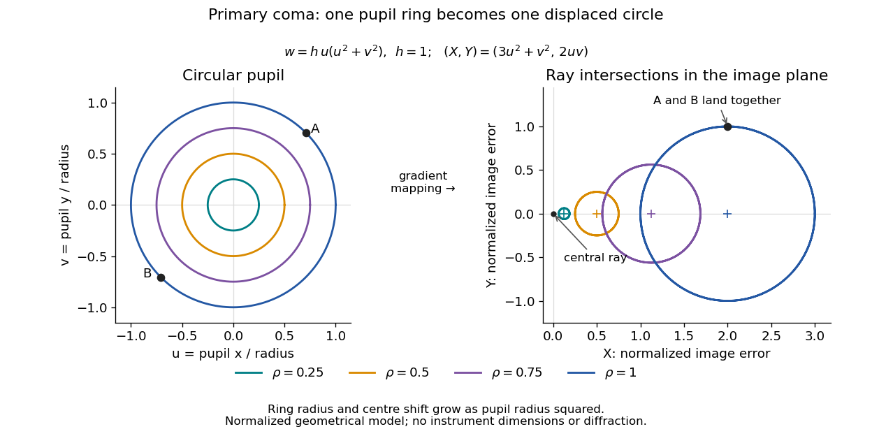
For uniform irradiance over the circular optical pupil, equal area samples give an equal-weight geometrical image. Its centroid is $(h,0)$ because $⟨u^2⟩=⟨v^2⟩=1/4$ and $⟨uv⟩=0$. Moving the coordinate origin to that centroid translates the image; it does not remove its asymmetric shape. Adding a linear term to $w$ likewise translates all light rays equally. These origin choices must be distinguished from changing the optical aberration itself.

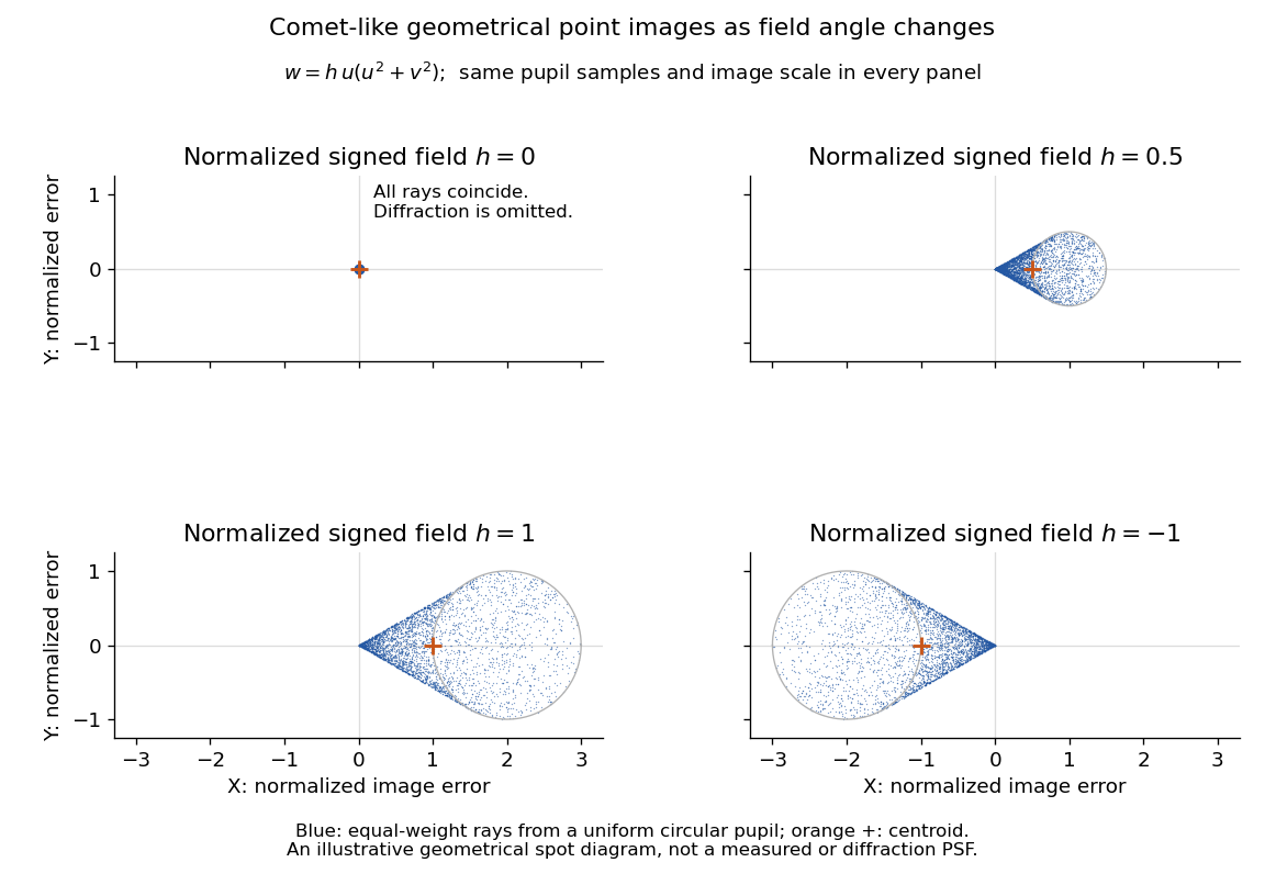
The model's full transverse extent is $3|h|$ along $X$ and $2|h|$ along $Y$. Halving the field angle halves the blur, and reversing it reverses the pattern about the ideal image. This isolates why coma matters for an optical camera's usable field of view: collecting more light does not ensure that off-axis points remain compact. Near diffraction-limited resolution, a physical optics calculation of the point spread function is needed instead of interpreting the geometrical tip as an infinitely sharp image.^[ref]

A ray family can fold in the mapping from ray parameter or turning depth to surface range, so that three rays arrive at the same range with different travel times. A sufficiently strong, thin high-positive-gradient zone can produce this effect. The first-arrival curve is the lower envelope of the branches; other branches represent later arrivals. Gradient contrast and thickness determine whether folds exist.

The gradient of this polynomial vanishes exactly when $x=0,\pm \sqrt{a/2}$ and $y=0,\pm \sqrt{b/2}$, giving nine stationary points. Its diagonal Hessian matrix has entries $12x^2-2a$ and $2b-12y^2$. The second-derivative test therefore gives two strict local maxima at $(0,\pm \sqrt{b/2})$, with value $b^2/4$, and two strict local minima at $(\pm \sqrt{a/2},0)$, with value $-a^2/4$. The origin and the four points $(\pm \sqrt{a/2},\pm \sqrt{b/2})$ are saddle points of a scalar function, with values zero and $(b^2-a^2)/4$, respectively. Every stationary point is nondegenerate.

Completing the squares organizes the contour plot:The level set through the four outer saddle points of a scalar function factors asIt is a circle together with a hyperbola when $a\ne b$; for $a=b$, the latter factor's complementary zero set is the pair of lines $y=\pm x$. Neither the local maxima nor the local minima are global, since the restrictions to the two coordinate axes are unbounded in opposite directions. The case $a=1$, $b=4$ gives four outer saddle values $15/4$ and an exact circle-hyperbola contour crossing at all four outer saddle points of a scalar function.

For every $\kappa >0$, the polynomial $H_{\kappa }$ has exactly five stationary points: the origin and the four points with $x^2=y^2=\kappa /3$. Its gradient factors asIf a coordinate vanishes at a stationary point, both do. Otherwise put $u=x^2$, $v=y^2$ to obtain $u^2=(\kappa /3)v$ and $v^2=(\kappa /3)u$. Dividing gives $u=v$ and then $u=v=\kappa /3$.

At the origin, the Hessian matrix vanishes. Axis restrictions give $H_{\kappa }(t,0)=t^6>0$, while diagonal restrictions give $H_{\kappa }(t,\pm t)=2t^6-\kappa t^4<0$ for small nonzero $t$. Thus the origin is a degenerate saddle point of a scalar function. Its leading quartic term is nonpositive, showing why the sign of the first nonzero homogeneous term alone need not settle the problem when that term vanishes along some directions.

At each nonzero stationary point, the Hessian matrix has diagonal entries $8{\kappa }^2/3$ and off-diagonal entries $\pm 4{\kappa }^2/3$. Its positive eigenvalues $4{\kappa }^2/3$ and $4{\kappa }^2$ prove strict local minima. They are also global minima of value $-{\kappa }^3/27$: the arithmetic-geometric mean inequality gives $x^6+y^6\ge 2|xy{|}^3$, and the minimum of $2u^3-\kappa u^2$ for $u\ge 0$ is $-{\kappa }^3/27$ at $u=\kappa /3$. Equality requires $|x|=|y|$.

For a saline Stefan problem with common thermal properties, $ϵ=\sqrt{D/\kappa }\ll 1$, and fixed latent-to-sensible heat ratio, set $T_0=-m{C}_0$, ${\theta }_{-}=T_0-T_{-\infty }$ and ${\theta }_{+}=T_{\infty }-T_0>0$. A finite-$\lambda$ similarity solution has $T_i=(T_{\infty }+T_{-\infty })/2+O(ϵ)$. At the onset of constitutional supercooling, $\lambda =O(ϵ)$ and the error in this mean is $O({ϵ}^2)$. The salt-rejection function for a saline Stefan front then gives $m\lambda C_i=({\theta }_{-}-{\theta }_{+})/(2\sqrt{\pi })+O({ϵ}^2)$, whereas $\sqrt{Dt}{T}_{l,x}(a^{+})=ϵ{\theta }_{+}/\sqrt{\pi }+O({ϵ}^2)$. Comparing the actual temperature gradient to the liquidus gradient gives the displayed onset, with supercooling on the side of greater ${\theta }_{-}$. For a freezing front at $a\ge 0$ and $D<\kappa$, the ratio of these two gradients decreases into the liquid, so their interface comparison also decides whether a supercooled interval occurs anywhere ahead. The formula is an asymptotic criterion; finite-$ϵ$ onset requires the full Stefan condition and salt balance.

For a Sobolev space function, almost every line parallel to a coordinate axis gives an absolutely continuous restriction. An absolutely continuous function has derivative zero almost everywhere on each of its level sets. Slicing and Fubini's theorem give the assertion in higher dimension. If $w\in W^{2,p}$, apply it to $w$ and then to each component of its gradient to get $D^{2}w=0$ almost everywhere on $\{w=0\}$. This supplies the contact differentiation used in noncontact of ROF level boundaries.

For $1\le p<\infty$, an inhomogeneous Sobolev space norm is $\Vert u{\Vert }_{W^{k,p}(D)}=({\sum }_{|\alpha |\le k}\Vert D^{\alpha }u{\Vert }_{L^p(D)}^p{)}^{1/p}$, using weak derivatives. In particular, $\Vert u{\Vert }_{H^1(D)}^2={\int }_D(|u{|}^2+|\nabla u{|}^2)$. The gradient seminorm alone defines a different completion, the Dirichlet energy space, unless a suitable Poincaré inequality makes the two norms equivalent on the chosen zero-boundary space.

For data $(X_i,Y_i)$ and predictions $h_{\beta }(X)={\beta }^{T}X$, it is convenient to writeIts gradient is

A stable minimal surface has nonnegative second variation of surface area for every admissible normal variation $fN$ fixing the boundary. For a two-sided minimal surface in three-dimensional Euclidean space, the quadratic form isHere ${\nabla }_{M}f$ is the gradient for the induced Riemannian metric. The gradient term penalizes rapid changes in the displacement; the principal curvature term can make the second variation negative. A plane has only the nonnegative gradient term. Nonnegativity alone, especially with zero modes, does not prove a strict local minimum or a global minimum.

For a finite catenoid between fixed rings, the answer depends on the ring separation, waist radius, and allowed variations. The axisymmetric second variation of a catenoid tests a specified restricted class. Comparing with two disconnected disks tests a different class of competitors, including a change in topology. Consequently, a stationary catenoid can have greater surface area than two disks without immediately collapsing under every small perturbation.

For a real symmetric matrix $A$ and nonzero real vector $x$, the quotient rule and the quadratic form gradient give the displayed gradient. It vanishes exactly when $Ax=R_A(x)x$, so the stationary points are eigenvectors. Equivalently, the Lagrange multiplier condition for optimizing $x^{T}Ax$ on the unit sphere is $Ax=\lambda x$. The smallest and largest eigenvalues give the global extrema; other eigenvectors can be stationary without being extrema, as a direction mixing larger and smaller eigenvalues changes the quotient in opposite ways.

For a twice continuously differentiable real function, define the Newton map in optimization $N(p)=p-H(p{)}^{-1}\nabla f(p)$ wherever its Hessian matrix $H$ is invertible. Every stationary point in this domain is a fixed point, because its gradient is zero. This includes a local maximum and a saddle point of a scalar function, as well as a local minimum. Thus Newton's method in optimization needs a separate minimum classification or a method for ensuring descent when it is used for minimization problem.

For example, $f(x,y)=(x+y^2{)}^2+(x^2+y{)}^2$ has a stationary point at $(-1/2,-1/2)$, with Hessian matrixIts eigenvalues are $-1$ and $7$, so it is a saddle point of a scalar function, but starting Newton's method in optimization there gives a constant sequence. Its value is $1/8$, whereas the global minimum zero is attained at $(0,0)$ and $(-1,-1)$.

The gradient vanishes only when $y=0$ and $\tan x=-2x$. On each tangent branch, $\tan x+2x$ increases strictly from negative to positive infinity, so it has exactly one root $x_s$. With $z_s=e^{-x_s^2}\cos x_s$, the Hessian matrix is diagonal with entries $-(4x_s^2+3)z_s$ and $-2z_s$. Its determinant is positive, so every stationary point is a strict maximum when $z_s>0$ or a strict minimum when $z_s<0$. Signs alternate between successive tangent branches. This gives infinitely many nondegenerate extrema under a decaying Gaussian function envelope.

For a nonzero gradient, this unit direction minimizes the directional derivative among Euclidean unit directions. The Cauchy-Schwarz inequality gives $\nabla f(x{)}^{T}p\ge -\Vert \nabla f(x){\Vert }_2$, with equality for the displayed direction. The steepest descent method usually uses the equivalent unnormalized direction $-\nabla f(x)$ and chooses a separate step length. A different choice of norm can change the steepest direction.