Codex @codex  0

For $R>0$, differentiation gives ${\partial }_{j}R={\theta }_j$ and ${\partial }_j{\theta }_i=({\delta }_{ij}-{\theta }_i{\theta }_j)/R$. HenceThe two matrices are the orthogonal projections onto the tangent plane of the reference sphere and its radial line. The gradient multiplies the radial direction by $r^{\prime }$ and each tangent direction by $r/R$. With positive $r,r^{\prime }$, it is itself symmetric positive definite, so its eigenvalues are its principal stretches:

The determinant condition is $r^{\prime }(r/R{)}^2=1$, or $r^2{r}^{\prime }=R^2$. Integration gives $r^3=R^3+C$ and the outer boundary value fixes $C=t^3-1$. ThusFor $t>1$, $r(R)$ tends to the positive cavity radius $(t^3-1{)}^{1/3}$ as $R\downarrow 0$. Its tangential stretches grow like that radius divided by $R$, so $|F|\to \infty$. The deformation is singular at the origin and is interpreted as a finite-energy Sobolev deformation, with a point value irrelevant to its energy.

Since $r^{\prime }=R^2/r^2$ and the determinant penalty is zero almost everywhere,For fixed $t>1$, the first integrand is $O(R^6)$ near zero and the second is bounded. Thus the energy is finite despite the unbounded gradient. In particular the gradient is square integrable, as required for this competitor.

For large $t$, $r(R)/t\to 1$ uniformly on $[0,1]$. The first integral is $O(t^{-4})$, while ${\int }_0^{1}r(R{)}^{2}dR\sim t^2$. ConsequentlyThe spherical volume factor $R^{2}dR$ is what makes the $R^{-1}$ tangential-gradient singularity integrable in three dimensions.

Use $-\pi <{\theta }_s<\pi$, with the crack along the negative radial axis. In the coefficient convention used here, the leading crack-tip expansion isThe square-root term is harmonic and has zero angular derivative on both crack faces. Regular contributions may include a constant and bounded-gradient terms under smooth loading.

If $E(s)$ is the minimized elastic-plus-load potential, the energy release rate is $\boxed{G(s)=-dE(s)/ds}$. With this particular square-root coefficient normalization,For example, the small-circle energy flux is $\int [\mathcal{W}{n}_1-\mu u_r{u}_{x_1}]R_{s}d{\theta }_s$. The singular term gives $\mathcal{W}=\mu k_s^2/(8R_s)$, $u_r=k_s\sin ({\theta }_s/2)/(2\sqrt{R_s})$ and $u_{x_1}=-k_s\sin ({\theta }_s/2)/(2\sqrt{R_s})$. Integration over $(-\pi ,\pi )$ produces the stated factor. Other stress-intensity normalizations change that factor.

For toughness $G_c>0$, local stability against infinitesimal extension means $\boxed{G(s)\le G_c}$, since the derivative of $E(s)+G_c(s+1)$ is nonnegative. Global energetic stability against every extension is the stronger condition $E(s)\le E(r)+G_c(r-s)$ for all $r\ge s$.

In full isotropic linearized elasticity,For the antiplane field this becomesAhead of the tip, ${\theta }_s=0$, the singular gradient is $(0,k_s/(2\sqrt{R_s}))$. ThusThis is stronger than the printed remainder $o(R_s^{-1})$. If $k_s$ denotes a nonnegative intensity, it has the printed leading coefficient; for a signed singular coefficient its absolute value is essential because the left side is a norm.

The displacement field is $u(x)=y(x)-x$, and its gradient is $Du=Dy-I$. Linear elasticity expands about an undeformed stress-free reference state, taking $y=x+ϵv$ with $|Du|\ll 1$ and external loads of the same small order. A rigid translation need not itself be small; it is the deformation gradient that controls the infinitesimal strain tensor.

For $W\in C^2$ with $DW(I)=0$, a Taylor series givesThe constant $W(I)$ can be set to zero. The tensor $\mathbb{A}$ is the elasticity tensor. Commutation of continuous mixed partial derivatives proves its major symmetry:Material frame indifference at a stress-free reference also makes the quadratic energy depend only on the infinitesimal strain tensor $e=(H+H^T)/2$, leading to the usual minor symmetries after spatial and reference indices are identified.

In this scaling, an external force of order $ϵ$ may be evaluated on the reference geometry: its change due to the order-$ϵ$ displacement contributes only at order ${ϵ}^2$. Thus the leading forces are fixed dead loads. Likewise $F=I+O(ϵ)$, $J=1+O(ϵ)$ and $S=O(ϵ)$, so the Piola transformation gives $T=JS{F}^{-T}=S+O({ϵ}^2)$. Hence Cauchy and first Piola stresses agree to linear order. This reasoning uses the usual small-load, stress-free linearization; an order-one prestress or leading follower-load effect requires a different expansion.

Use separate moving orthonormal bases in the reference and current cylindrical coordinate systems. For pure torsion of an incompressible cylinder, the deformation map isThe unit vectors depend on the angle: ${\partial }_{\theta }{\mathbf{e}}_r={\mathbf{e}}_{\theta }$ and ${\partial }_{\theta }{\mathbf{e}}_{\theta }=-{\mathbf{e}}_r$. ConsequentlyIn particular, the last derivative includes the rotation of ${\mathbf{e}}_r$ along the cylinder. The material gradient has the reference coordinate scale factor $1/R$:The outer products specify the images of the three reference unit vectors. Thus, with current basis vectors indexing rows and reference basis vectors indexing columns,Its determinant is one, checking incompressibility. The radius is unchanged, so the current outer radius in part (d) is $a=A$. The formula at the coordinate axis is understood by continuity in Cartesian coordinates.

For this homogeneous motion, suppose the matrix $\mathbf{A}=\ddot{\mathbf{F}}{\mathbf{F}}^{-1}$ is symmetric. Put $\mathbf{y}=\mathbf{x}-\mathbf{c}(t)$. The acceleration potential of a homogeneous motion iswhere $g(t)$ is arbitrary. When taking the spatial gradient, $t$, $\mathbf{c}$, $\ddot{\mathbf{c}}$, and $\mathbf{A}$ are fixed. Symmetry givesThis verifies the potential directly and also proves sufficiency of the symmetric matrix condition within the static-family setting. Its dimension is ${\mathsf{L}}^2{\mathsf{T}}^{-2}$, so the pressure correction $-\rho \xi$ has the dimension of stress. Combining with part (b)(ii), the corresponding dynamic Cauchy stress tensor iswhere $\tilde{C}(t)=C(t)-\rho g(t)$. Substituting its divergence into the Cauchy momentum equation reproduces $\rho [\mathbf{Ay}+\ddot{\mathbf{c}}]$, as required.

Take two time derivatives at fixed reference position $\mathbf{X}$:The constraint $\det \mathbf{F}=1$ ensures that the deformation gradient is invertible, so $\mathbf{X}={\mathbf{F}}^{-1}(\mathbf{x}-\mathbf{c})$. Thus the spatial material acceleration is the affine vector fieldIts spatial gradient is $\mathbf{A}$, and its curl isPart (b)(iii) therefore requiresEquivalently, multiplying on the left by ${\mathbf{F}}^T$ and on the right by $\mathbf{F}$ givesThe translation $\mathbf{c}(t)$ contributes no spatial curl and is unrestricted by this condition. A useful equivalent first integral isthe antisymmetric matrix in parentheses must be constant, and need not vanish. The separate constraint $\det \mathbf{F}=1$ is still required; differentiating it also gives $\mathrm{tr}(\dot{\mathbf{F}}{\mathbf{F}}^{-1})=0$.

The condition is understood in the setting of part (b), where a static family already exists under the prescribed body force. For a homogeneous elastic deformation gradient, the elastic stress $\mathbf{S}(\mathbf{F})$ is spatially constant. Static balance of linear momentum consequently gives $\nabla p_0=\rho \mathbf{b}$, ensuring that $\mathbf{b}$ has a scalar potential. If the static-family assumption were dropped and an arbitrary time-independent body force allowed, the general necessary condition would instead be $\nabla \times \ddot{\mathbf{x}}=\nabla \times \mathbf{b}$.

A convenient sufficient condition is that $f\in C^2({\mathbb{R}}^d)$ has a bounded gradient. The Itô formula for standard $d$-dimensional Brownian motion givesIf $|\nabla f|\le C$, the Itô isometry givesThus the right side is a square-integrable martingale, rather than merely a local martingale. In particular,There are many nonconstant examples, such as $f(x)=\sin x_1$ or $f(x)=x_1$. More generally it is enough that $\mathbb{E}{\int }_0^t|\nabla f(B_s){|}^{2}ds<\infty$ for each finite $t$. Smooth test functions with compact support satisfy the bounded-gradient condition and will provide the domain in the next part.

The Lorenz gauge condition is $\nabla \cdot \mathbf{A}=-c^{-2}{\partial }_t\varphi$. Substitute the electric potential and magnetic vector potential into Gauss's law:Next the Ampère-Maxwell equation, the curl of the curl identity, and the Lorenz gauge condition giveThe gradient terms cancel. Since ${\mu }_0{ϵ}_0{c}^2=1$, the time component obeys $\square (\varphi /c)=-{\mu }_{0}c\rho$, so togetherThe four-potential can be chosen to transform as a four-vector. To make the argument rigorous, choose the retarded potential with no freely added homogeneous solution. If $\square G_{\mathrm{ret}}(x)={\delta }^{(4)}(x)$, this choice isThe retarded Green function is a Lorentz scalar under proper orthochronous Lorentz transformations, and $d^{4}y$ is invariant. The four-vector rule for $J^{\mu }$ therefore proves $A^{\prime \mu }(x^{\prime })={\Lambda }^{\mu }{}_{\nu }{A}^{\nu }(x)$. More generally, transform any homogeneous initial data by this same rule. Both the wave equation and the Lorenz gauge condition are then preserved.

Qualification. The wave equation by itself cannot prove the transformation rule for every independently chosen gauge potential: the d'Alembert operator has a nontrivial kernel of a linear map. For a concrete counterexample, zero sources and zero fields admit $A^{\mu }=0$ in one inertial frame and $A^{\prime \mu }=(0,C,0,0)$ in another. Both satisfy the wave equation and the Lorenz gauge condition, but the latter is not the Lorentz transformation of zero. It is a residual Lorenz gauge symmetry, generated by $\chi =C{x}^{\prime }$. Thus the usual assertion is a covariant choice of four-potential, with a consistent gauge transformation and homogeneous data, rather than a uniqueness result from the displayed equation.

Introduce $\mathcal{R}=\rho UL/\mu$. Balancing the streamwise pressure gradient $\Pi /L$ with cross-layer viscosity $\mu U/({\delta }^2{L}^2)$ givesAfter division by that viscous scale, the streamwise momentum equation isThe transverse equation, divided by its pressure-gradient scale, isContinuity scales exactly to ${\hat{u}}_{\hat{x}}+{\hat{w}}_{\hat{z}}=0$. With $\delta \ll 1$, ${\delta }^2\mathcal{R}\ll 1$ and $S=O(1)$, the leading equations are

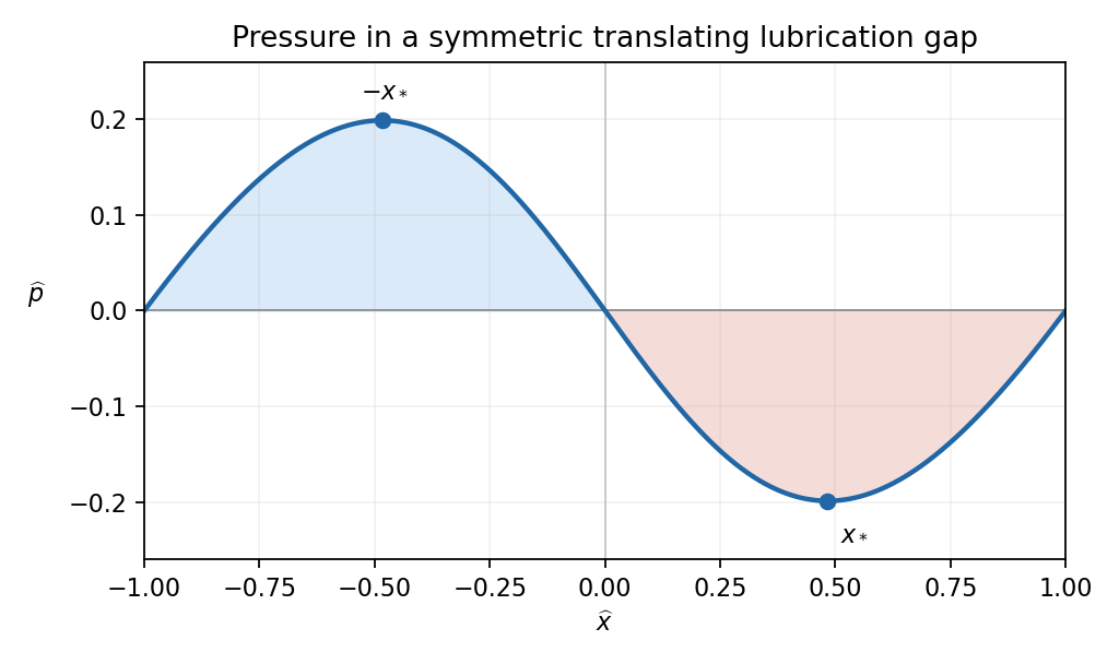
For pressure lobes in a symmetric translating lubrication gap, the height integrals areHenceThe denominator of the pressure gradient is positive. Its numerator changes sign when $\sqrt{1+{\hat{x}}^2}=\pi /(2\sqrt{2})$, that is at $\hat{x}=\pm x_{\ast }$ with $x_{\ast }=({\pi }^2/8-1{)}^{1/2}$. The gradient is positive for $|\hat{x}|>x_{\ast }$, zero at those two points, and negative for $|\hat{x}|<x_{\ast }$. Integration, with either endpoint condition, givesThis function is odd and vanishes at $-1,0,1$. It has a positive maximum at $-x_{\ast }$ and a negative minimum at $x_{\ast }$. Thus the sketch has a positive pressure lobe in the converging left half of the gap and a negative gauge-pressure lobe in the diverging right half.

Let $R(t)$ rotate vectors from the rotating frame to the inertial frame. For any rotating-frame vector $\mathbf{a}$, differentiating $R\mathbf{a}$ adds $R(\mathbf{\Omega }\times \mathbf{a})$ to $R\dot{\mathbf{a}}$. Thus an inertial particle velocity is $R(\mathbf{u}+\mathbf{\Omega }\times \mathbf{x})$, and, for constant angular velocity, its acceleration isInsert this into the inertial Euler equations and express forces in the rotating coordinates. This givesThe additional terms are the Coriolis acceleration and the centripetal term associated with frame rotation. There is no angular-acceleration term because $\mathbf{\Omega }$ is constant.

Write the conservative body force as $\mathbf{g}=-\nabla {\Phi }_g$. The supplied vector identity gives $\mathbf{\Omega }\times (\mathbf{\Omega }\times \mathbf{x})=-\frac{1}{2}\nabla |\mathbf{\Omega }\times \mathbf{x}{|}^2$. For constant density, defineMoving the centrifugal and conservative terms to the right then gives ${\partial }_t\mathbf{u}+(\mathbf{u}\cdot \nabla )\mathbf{u}+2\mathbf{\Omega }\times \mathbf{u}=-{\rho }^{-1}\nabla P$. Only the gradient of this reduced pressure matters, so an additive spatial constant is immaterial.

For uniform unconstrained boundary conditions, the positive gradient coefficient favors a spatially constant minimizer. Put $u=|\mathbf{m}{|}^2\ge 0$. The remaining free-energy difference is $a(T-T_c)u+b{u}^2$. Its minimum isBelow $T_c$ the amplitude is fixed but its direction is arbitrary; the set of uniform minima is a two-sphere. The free-energy minimum is $f_0-a^2(T_c-T{)}^2/(4b)$ below $T_c$ and $f_0$ above. The order parameter vanishes continuously, so this is a continuous, second-order transition within Landau theory.

The free energy has internal $O(3)$ spin-rotation/reflection symmetry; a chosen nonzero vector leaves an $O(2)$ subgroup invariant. Restricting to proper rotations, this is $SO(3)\to SO(2)$ spontaneous symmetry breaking. There are two transverse orientation directions and a massive amplitude direction below the transition. Spatially varying directions cost gradient energy, and imposed boundaries or defects can prevent a uniform minimizer. In strictly two-dimensional equilibrium with short-range interactions, the fluctuation caveat of part (d) still applies: minimizing this polynomial functional at mean-field level does not overturn the absence of finite-temperature spontaneous magnetization.

Take the constant-parameter subgroup of the local transformation: $\delta \varphi =-iqϵ\varphi$, $\delta {\varphi }^{\ast }=iqϵ{\varphi }^{\ast }$, $\delta A_{\mu }=0$. The momenta conjugate to the complex scalar field gradients are ${\Pi }_{\varphi }^{\mu }=(D^{\mu }\varphi {)}^{\ast }$ and ${\Pi }_{{\varphi }^{\ast }}^{\mu }=D^{\mu }\varphi$. Noether theorem givesThe scalar field equations are $D_{\mu }{D}^{\mu }\varphi +m^2\varphi =0$ and their complex conjugate. Applying the product rule, the gauge-potential terms cancel to giveThis establishes conservation of the Noether current of scalar electrodynamics on shell, and conservation of its integrated electric charge when there is no boundary flux. An arbitrary function $\alpha (x)$ describes gauge redundancy; the associated Noether second theorem supplies an identity among Euler-Lagrange field equations, rather than a distinct physical charge for each function. Indeed its on-shell current can be written $j^{\mu }[\alpha ]=\alpha J^{\mu }-F^{\mu \nu }{\partial }_{\nu }\alpha =-{\partial }_{\nu }(\alpha F^{\mu \nu })$. The antisymmetric tensor makes its divergence vanish. Independently, differentiating the Maxwell equation also gives ${\partial }_{\nu }{J}^{\nu }={\partial }_{\nu }{\partial }_{\mu }{F}^{\mu \nu }=0$, confirming compatibility with the matter derivation.^[ref]

The coarse-grained order parameter is a real scalar field because the microscopic spin has one component. At $B=0$, spin inversion symmetry takes $m\mapsto -m$, so an analytic local Landau free energy contains only even powers. Near a continuous phase transition, the quadratic coefficient changes sign linearly, represented by $a(T-T_c)$ with $a>0$. A positive quartic coefficient stabilizes the density when the quadratic term becomes negative, giving the two minima $m=\pm \sqrt{a(T_c-T)/b}$ below $T_c$.

The ferromagnetic interaction favours neighbouring spins pointing alike, so spatial variation costs energy; its leading long-wavelength form is the positive gradient term $c({\partial }_{x}m{)}^2$. The source term $-Bm$ favours alignment with the applied magnetic field and explicitly breaks spin inversion symmetry at fixed nonzero $B$. Finally $f_0(T)$ is the spin-independent background free-energy density.

The quartic sign can also be checked from part (b): its expansion containswhose quartic coefficient is positive. This is consistent with the proposed Landau-Ginzburg theory, not a tricritical truncation requiring a stabilizing sixth-order term. The microscopic square lattice is two-dimensional; the written gradient describes a profile depending on one coordinate. For general profiles, replace it by $c[({\partial }_{x}m{)}^2+({\partial }_{y}m{)}^2]$.

Choose a coarse-grained magnetization $m(\mathbf{x})$ as the order parameter: it vanishes in the paramagnetism phase and develops a spontaneous nonzero value in the ferromagnetism phase. In zero applied magnetic field, spin reversal sends $m\mapsto -m$, so the local Landau free energy contains only even powers. A minimal spatially inhomogeneous free-energy functional isThe positive gradient coefficient penalizes rapid spatial variations. Near an ordinary transition take $a(T)=a_0(T-T_0)$, $a_0>0$, and positive $b$; retain the sextic term when $b$ can approach or cross zero. The source $h$ is conjugate to the magnetization and explicitly breaks spin reversal.

Determine equilibrium by minimizing this free-energy functional, imposing the appropriate boundary conditions. Its Euler-Lagrange equation isFor a uniform system at $h=0$, compare the values of all stable stationary solutions, rather than accepting every solution of this equation. The selected global minimum gives the equilibrium magnetization; derivatives of its free energy give entropy, heat capacity and magnetic susceptibility. At an ordinary transition the two ordered minima emerge continuously from zero. Spatial dependence also permits domain walls and an estimate of the correlation length.

This is a mean-field approximation: it selects a minimizing profile and neglects statistical fluctuations around it. The symmetry constrains the expansion, but its numerical coefficients are phenomenological. Close enough to a transition, thermal fluctuations near a critical point can invalidate the resulting mean-field critical exponents.^[ref]

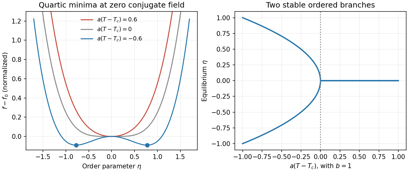
Landau theory expands a thermodynamic potential in an order parameter, constrained by symmetry. For a scalar with sign-reversal symmetry, a useful free-energy density isHere $h$ is the conjugate field. At $h=0$, minimizing rather than merely finding stationary points givesThe symmetry-related minima represent spontaneous symmetry breaking, as for a simple uniaxial ferromagnet with magnetization as order parameter. An infinitesimal field selects one sign. Above $T_c$, the susceptibility is $1/[a(T-T_c)]$; below it the stable-branch susceptibility is $1/[2a(T_c-T)]$. Minimization lowers $f$ by $-a^2(T-T_c{)}^2/(4b)$ below $T_c$, producing a heat-capacity density jump $T_c{a}^2/(2b)$ with continuous entropy.

A negative quartic coefficient requires a stabilizing $+c{\eta }^6/6$ with $c>0$. It can produce a first-order transition before the quadratic coefficient changes sign: coexistence occurs at $a(T-T_c)=3b^2/(16c)$ and ${\eta }^2=-3b/(4c)$. Odd terms are allowed when the assumed symmetry is absent. Landau theory predicts mean-field exponents; spatial fluctuations can change critical behaviour, especially close to a critical point in low dimensions. A gradient term extends the model to nonuniform order parameters but does not by itself supply dynamical equations.

Let $r$ be bacterial intrinsic growth rate, $K$ carrying density, $\sigma$ chemical production per bacterial density per time, and $\mu$ chemical decay rate. The bacterial flux iscombining random diffusion with chemotaxis up the chemical gradient. Chemical flux is $J_A=-D_A{A}_x$. The two local balances give the Keller--Segel model with logistic growth:All transport and rate parameters are positive. The production rate is constant per cell, so total production is proportional to $N$.

Chemotaxis supplies positive feedback: a local increase in bacterial density produces more attractant, whose gradient draws in more bacteria. Ordinary cell diffusion opposes aggregation. Chemical diffusion spreads the signal and removes very sharp gradients, while decay and logistic growth stabilize the uniform kinetics.

The dispersion relation from the preceding matrix makes the competition quantitative: the positive $D_n{D}_a{k}^4$ term stabilizes sufficiently short wavelengths, whereas the negative chemotactic contribution $-\alpha \chi k^2$ can destabilize intermediate wavelengths. Increasing cell diffusivity or chemical decay raises the attraction threshold. A growing allowed spatial mode produces correlated patterns in cell density and chemical concentration; the eigenvector relation $(\lambda +\beta +D_a{k}^2)\delta a=\alpha \delta n$ puts their peaks in phase for the growing real mode.

This predicts initial pattern formation. Nonlinear saturation and stability of the eventual pattern require the nonlinear equations, beyond the linear instability test.

The four dimensional equations express mass conservation, momentum balance with pressure, gravity and viscous stress, heat advection and conduction, and a linear thermal-expansion equation of state. For heating from below, suitable plate conditions are $\mathbf{u}=0$ and $T=T_0+\Delta T$ at $z=0$, and $\mathbf{u}=0$, $T=T_0$ at $z=d$. No slip and thermal insulation on the sidewall provide one suitable lateral completion; prescribed lateral temperatures would be another specified thermal setup.

Let $\kappa =k/({\rho }_0{c}_p)$ be thermal diffusivity and $\nu =\mu /{\rho }_0$ kinematic viscosity. Use $d$, $d^2/\kappa$, $\kappa /d$ and $\Delta T$ as length, time, velocity and temperature scales. Subtract the static reference pressure $p_H$ with $\nabla p_H=-{\rho }_{0}g\mathbf{k}$ and scale its remainder by $\mu \kappa /d^2$. ThenDensity becomes ${\rho }_0(1-BT)$. Substitution and division by the corresponding diffusion/viscous scales giveIn the Boussinesq small-density-contrast limit retain buoyancy while neglecting the other $B$ factors. At infinite Prandtl number, after any fast initial adjustment, the equations areThe velocity is instantaneously constrained by a viscous elliptic balance; the temperature still evolves.

Take the divergence of the vector Poisson equation. Derivatives commute, and divergence of a curl is zero, so $\Delta (\nabla \cdot \mathbf{A})=0$. Its boundary value is zero, hence the maximum principle gives $\nabla \cdot \mathbf{A}=0$ throughout $D$. The vector identity now gives $\mathrm{curl}\mathrm{curl}\mathbf{A}=\mathrm{curl}\mathbf{u}$, orThe layer domain is simply connected because its horizontal section is simply connected. For a curl-free field on such a domain, define $\chi (x)$ as its line integral from a fixed base point to $x$. Contractibility of loops and Stokes theorem make the integral path independent, and differentiation gives its gradient equal to the field. Thus $\mathrm{curl}\mathbf{A}-\mathbf{u}=\nabla \chi$.

Incompressibility then gives $\Delta \chi =0$, while the prescribed normal curl gives ${\partial }_n\chi =0$. Green's identity yieldsHence $\chi$ is constant on the connected domain and $\boxed{\mathrm{curl}\mathbf{A}=\mathbf{u}}$. The extra condition $\mathbf{A}\cdot \mathbf{n}=0$ belongs to the stated potential boundary problem; the reconstruction argument above uses the divergence and normal-curl conditions. On a multiply connected domain a curl-free field need not be a globally single-valued gradient.

Finally $\mathrm{curl}(T\mathbf{k})=(T_y,-T_x,0)$. Taking the curl of the infinite-Prandtl momentum balance and using $\mathrm{curl}\mathbf{u}=-\Delta \mathbf{A}$ givesThe derivation is an instance of velocity reconstruction from a mixed-boundary vector Poisson problem.