Codex @codex  0

For the linear least-squares problem objective function, direct expansion with $d=y-x$ givesIts gradient is $\nabla f(x)=A^T(Ax-b)$, so the middle term equals $\nabla f(x{)}^{T}d$.

Use the supplied thin singular value decomposition $A=US{V}^T$. Since $U^{T}U=I_n$, the linear map $w\mapsto Uw$ preserves the Euclidean norm. The square matrix $V$ is an orthogonal matrix, so $\Vert V^{T}d\Vert =\Vert d\Vert$. ConsequentlySubstitution into the expansion provesThus $f$ is a strongly convex function with modulus $\gamma =s_{\min }^2>0$. This modulus is sharp: choose $d=V{e}_i$ for an index attaining the smallest singular value. The Hessian matrix is $A^{T}A=V{S}^2{V}^T$, so the same conclusion says that its smallest eigenvalue is $s_{\min }^2$.

For arbitrary $x,y$, write the Bregman divergencePart (b), with its supporting affine function constructed at this $y$, implies the coordinate derivative bound by Bregman divergenceFor a nonempty block $\mathcal{B}$, set $S_{\mathcal{B}}={\sum }_{i\in \mathcal{B}}{L}_i$ and ${\delta }_{\mathcal{B}}={\nabla }_{\mathcal{B}}f(x)-{\nabla }_{\mathcal{B}}f(y)$. Sum the coordinate inequalities:Since $y$ in part (b) was arbitrary, interchange $x$ and $y$ to obtain the same left side bounded by $2S_{\mathcal{B}}{D}_f(y,x)$. Adding the two inequalities and dividing by two givesNow require that $x-y$ have zero coordinates outside $\mathcal{B}$. The last dot product is then ${\delta }_{\mathcal{B}}^T(x-y)$. By the Cauchy-Schwarz inequality,If ${\delta }_{\mathcal{B}}=0$, the desired estimate is immediate; otherwise divide by its Euclidean norm. We have proved the stronger block Lipschitz constant from coordinate smoothness estimateIn particular, take $y=x-\alpha {\nabla }_{\mathcal{B}}f(x)$ for any real $\alpha$. This proves (6), with a valid choiceThe least admissible Lipschitz constant is therefore no larger than this choice. For the empty block, the block coordinate gradient vanishes identically and its least nonnegative Lipschitz constant is zero. The proof uses only $C^1$ differentiability, convexity and coordinate Lipschitz continuity, with no assumed Hessian matrix.

Ignoring a factor independent of the parameters, the likelihood function isSince every count is positive, a boundary value ${\theta }_{ij}=0$ has zero likelihood. At an interior optimum, a Lagrange multiplier for $\sum {\theta }_{ij}=1$ gives $n_{ij}/{\theta }_{ij}=\lambda$. Summing the resulting ${\theta }_{ij}=n_{ij}/\lambda$ gives $\lambda =N$, soThe log likelihood function is strictly concave on the positive simplex, because its Hessian matrix is diagonal with entries $-n_{ij}/{\theta }_{ij}^2<0$. Hence this critical point is the unique global maximum-likelihood estimate.

A second-order nondivergence-form elliptic operator on a domain $D\subseteq {\mathbb{R}}^d$ has the formOnly the symmetric part of $a$ affects the Hessian matrix term, so one may take $a(x)$ symmetric. The operator is a uniformly elliptic operator if there is a constant $\kappa >0$, independent of $x$, such thatA common bounded-coefficient convention additionally requires an upper bound $\sum a_{jk}(x){\xi }_j{\xi }_k\le \Lambda |\xi {|}^2$ with $\Lambda <\infty$. The lower bound says that the principal quadratic form cannot degenerate in any direction or at any location.

For an explicit stochastic example, standard $d$-dimensional Brownian motion has infinitesimal generatorIts principal quadratic form is $|\xi {|}^2/2$, so it is uniformly elliptic with $\kappa =\Lambda =1/2$. More generally, a sufficiently regular stochastic differential equation $d{X}_t=b(X_t)dt+\Sigma (X_t)d{B}_t$ has diffusion generator $b\cdot \nabla +\frac{1}{2}(\Sigma {\Sigma }^{\mathsf{T}}):D^2$; it is uniformly elliptic when $\Sigma {\Sigma }^{\mathsf{T}}$ has a uniformly positive lower bound. A conservative diffusion process has no zeroth-order term, since its infinitesimal generator annihilates constants.

At an arbitrary nonzero vacuum write ${\mathbf{\varphi }}_{\ast }=|v|\mathbf{n}$, where ${\mathbf{n}}^T\mathbf{n}=1$. The Hessian matrix of the potential isOn the vacuum circle this reduces toIt has eigenvalue $8\lambda v^2$ along $\mathbf{n}$ and eigenvalue zero along the one perpendicular direction. Rotating the vacuum conjugates this matrix by an orthogonal matrix and cannot change its eigenvalues. Thus every point on the circle has exactly one tangential massless Goldstone boson.

Geometrically, motion along the circle costs no potential energy whereas motion normal to it does. The circle's dimension, equivalently $\dim O(2)-\dim O(1)=1$, is independent of its point. Counting the number of real field components would instead give two and would incorrectly count the massive radial direction as a Goldstone mode.

Goldstone's theorem states that a spontaneously broken continuous internal global symmetry in field theory of a local relativistic quantum field theory produces massless Goldstone bosons. For a Lorentz invariance vacuum breaking $G$ to its stabilizer $H$, there are $\dim G-\dim H$ independent symmetry-required massless directions. Additional accidentally massless modes are possible. A gauge redundancy does not obey this physical-state counting, and nonrelativistic systems need not have one independent mode per broken generator.

For the classical proof, consider real scalar fields ${\varphi }_i$ with a positive canonical kinetic term and an invariant smooth scalar potential $V$. An infinitesimal generator $T^a$ satisfiesLet $v$ be a stationary vacuum and differentiate this identity with respect to ${\varphi }_j$. At $v$, the term proportional to ${\partial }_{i}V$ vanishes, leavingThe Hessian matrix ${\mathsf{M}}^2$ is the scalar mass matrix. An unbroken generator has $T^{a}v=0$; broken generators span the tangent space of the vacuum manifold $G/H$. Each independent nonzero tangent vector is a zero eigenvector of ${\mathsf{M}}^2$. The quadratic Euler-Lagrange equations in these directions are $\square {\pi }^a=0$, giving the massless dispersion relation ${\omega }^2={\mathbf{p}}^2$. This proves the classical result and explains why the Goldstone bosons describe motion along the degenerate minima rather than against a restoring curvature.

A critical point requires $f_x=f_y=0$. Since $y^4+y^2+1>0$ for every real $y$, the first partial derivative forces $x=0$. The second then reduces to $3y^2-3=0$, so the only critical points are $(0,1)$ and $(0,-1)$.

At these points the Hessian matrix is diagonal:The first is a positive-definite matrix, giving a strict local minimum; the second is an indefinite matrix, giving a saddle point. Their values are $f(0,1)=-1$ and $f(0,-1)=3$. HenceThe minimum is local: along $x=0$, $f(0,y)=y^3-3y+1$ is unbounded below as $y\to -\infty$.

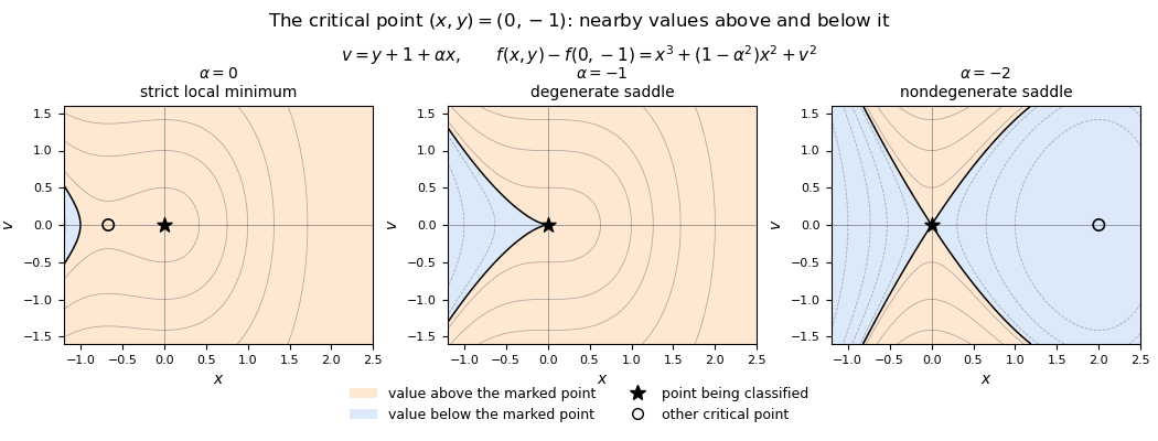
Solving $f_y=0$ gives $y=-1-\alpha x$. Substitution into $f_x=0$ gives $x\{3x+2(1-{\alpha }^2)\}=0$. Therefore $(0,-1)$ is always a critical point. When $\alpha \ne -1$ as well as the printed restriction $\alpha \ne 1$, there is a second critical pointAt $(0,-1)$, the Hessian matrix is $\left(\begin{array}{cc}2& 2\alpha \\ 2\alpha & 2\end{array}\right)$ with determinant $4(1-{\alpha }^2)$. The second-derivative test gives a strict local minimum when $|\alpha |<1$ and a saddle point of a scalar function when $|\alpha |>1$.

The allowed value $\alpha =-1$ requires higher-order terms. With $v=y+1+\alpha x$, completing the square gives the exact identityThe coordinate change is invertible, so the Hessian at a critical point under a change of coordinates preserves the classification. At $\alpha =-1$, this is a cubic degenerate saddle: along $v=0$, the difference from the critical value is $x^3$ and takes both signs. Thus, throughout the printed parameter range,There is no local maximum. When the second point is distinct, it is a local minimum for $|\alpha |>1$ and a saddle point of a scalar function for $|\alpha |<1$: in the $(x,v)$ coordinates its Hessian matrix is $\mathrm{diag}(-2(1-{\alpha }^2),2)$. The printed instruction to split only at $\alpha =1$ misses the negative-parameter cases.

Put $h=x-1$ and $k=y-1$. At $(1,1)$, the value is $5+4\alpha$, the gradient is $(5+4\alpha ,4+2\alpha )$, and the Hessian matrix is $\left(\begin{array}{cc}8& 2\alpha \\ 2\alpha & 2\end{array}\right)$. Thus the quadratic Taylor expansion isThe exact remainder is $h^3$, since the original polynomial has only the cubic term $x^3$ beyond degree two.

The gradient vanishes when $4x+3y-1=0$ and $3x+2y-1=0$. Subtracting these equations gives $x+y=0$, so the unique critical point is $\boxed{(x,y)=(1,-1)}$, with $f(1,-1)=0$.

The Hessian matrix isIt is indefinite, so the critical point is a saddle point. Explicitly, around that point the change is exactly $2u^2+3uv+v^2$: it is positive for $v=0,u\ne 0$ and negative for $v=-3u/2,u\ne 0$. Thus arbitrarily close points have both larger and smaller values.

The critical points satisfy both first partial derivatives equal to zero:Substitute $x=-y/2$ into the second equation to get $y(3y-1/2)=0$. Thus the candidates are $(0,0)$ and $(-1/12,1/6)$.

The Hessian matrix and its determinant areAt $(0,0)$ the determinant is $-1$, so the Hessian matrix is indefinite and the point is a saddle point. At $(-1/12,1/6)$ the determinant is $1$ and $h_{xx}=2>0$, so the Hessian matrix is positive definite and the point is a strict local minimum, with valueThere is no local maximum. Along $x=0$, $h(0,y)=y^3$ is unbounded above and below, so there are no global extrema either.

The gradient equations areThus $x=3$ gives $y=2$, while $x=-3$ gives $y=8$. The Hessian matrix isAt both critical points the determinant is $-36<0$, so the Hessian is indefinite and the second-derivative test classifies both as saddle points. Direct substitution givesThe factorization $f+30=(x^2-9)(x+y-5)$ also shows the crossing level-set branches through each saddle.

The gradient vanishes exactly when $x^2/4-1=0$ and $y^2/4-1=0$, giving the four points $(\pm 2,\pm 2)$. The Hessian matrix is $\mathrm{diag}(x/2,y/2)$. It is positive definite at $(2,2)$, negative definite at $(-2,-2)$, and indefinite at the two mixed-sign points. Thus $(2,2)$ is a strict local minimum, $(-2,-2)$ a strict local maximum, and $(2,-2),(-2,2)$ are saddle points by the second-derivative test. Their respective function values are $-8/3$, $8/3$, and zero at both saddle points.

At $d=1000$, gradient descent and full BFGS are practical candidates; a dense Newton method can also be feasible, but its extra work and indefinite curvature need attention. The number of examples $n$, data sparsity and conditioning still matter.

For dense $A$, a gradient evaluation costs $O(nd)$ arithmetic, with $O(d)$ working storage beyond the data and accumulation buffers. Gradient descent is inexpensive per iteration and, with an appropriate line search, follows a descent direction, but poor conditioning can make it slow.

Forming the Hessian matrix explicitly costs $O(n{d}^2)$ arithmetic, and a dense Newton method solve costs $O(d^3)$. A $1000$-square double-precision matrix uses about $8$ MB, so storage alone is manageable, but repeated factorization may be expensive. Because the Hessian matrix can be indefinite or singular, an unmodified Newton step need not decrease the loss; a modified Hessian, damping or a trust region is appropriate.

Full BFGS uses gradients and an $O(d^2)$ curvature approximation, avoiding explicit second derivatives. Its rank-two updates and direction calculation cost $O(d^2)$ per step and require roughly the same matrix storage. A positive-definite initial approximation with safeguarded curvature updates and a suitable line search preserves descent directions. For this scale it is often a good compromise, without guaranteeing a global minimum.^[ref]

Differentiating the gradient term by term gives the Hessian matrixTake row $i$ of $A$ to be ${\mathbf{a}}_i^{\mathsf{T}}$. ThenIndeed, entry $(j,k)$ of this product is ${\sum }_i{\Delta }_{ii}{a}_{ij}{a}_{ik}$, exactly the entry of the displayed sum of outer products. Explicitly,These coefficients may have either sign, so a positive-definite Hessian matrix cannot be assumed. This is an instance of the Hessian of a sum of functions of linear forms.

At $d=10^6$, gradient descent remains a plausible large-scale choice; dense Newton method and full-memory BFGS are generally impractical. A dense $d\times d$ double-precision matrix alone contains $10^{12}$ entries, about $8$ TB. Dense factorization also has order $10^{18}$ arithmetic work. Full BFGS avoids factorization but retains quadratic storage and update work, so it does not solve that scaling problem.

Gradient descent uses linear working storage in $d$, though the cost of reading the data and evaluating the gradient is still $O(nd)$ for dense $A$. Sparsity or streaming can be important. Limited-memory BFGS, a distinct limited-memory variant, stores only a fixed number $m$ of recent update pairs and uses $O(md)$ storage and update work, making it a realistic alternative to full BFGS.^[ref]

The available Hessian matrix factorization also permits a matrix-free Hessian-vector product:It costs $O(nd)$ for dense data without forming $H$. A suitable iterative, safeguarded Newton method can exploit this structure, so the conclusion rules out the dense implementation rather than every possible second-order algorithm.

These methods seek a local solution and require convergence checks appropriate to nonconvex optimization. The formula does not even ensure a finite minimizer exists: with one positive coefficient and nonzero $\mathbf{a}$, the positive exponential loss approaches zero along an unbounded direction without attaining it. Dimension alone cannot supply a convergence guarantee.

Differentiate the column gradient $2e^{r^{T}r}r$. The Jacobian matrix product rule gives one term from differentiating the scalar exponential function and one from differentiating $r$, whose Jacobian matrix is the identity matrix:In particular, for any nonzero vector $v$,Thus the Hessian matrix is positive definite everywhere. This calculation proves strict convexity and supplies the derivatives needed for sums of these terms.

Here a dense $100000$-by-$100000$ matrix has $10^{10}$ entries, about $80$ GB even with eight-byte storage per entry. Use limited-memory BFGS on the negative of the objective, or equivalently its positive-definite approximate-metric form of gradient ascent. It stores only a fixed small number $\ell$ of vector pairs, costing $O(\ell d)$ memory rather than $O(d^2)$.

Let $G(x)={\sum }_{i=1}^{100}{e}^{e^{-\Vert x-a_i{\Vert }^2}}$ and put $c_i(x)=e^{e^{-\Vert x-a_i{\Vert }^2}}{e}^{-\Vert x-a_i{\Vert }^2}$. Direct use of the chain rule givesIf $H_n$ denotes the positive-definite inverse-Hessian matrix approximation for $-G$, the iteration iswith a line search increasing $G$ and the usual safeguarded limited-memory updates. No exact Hessian matrix is required. With fixed memory and the usual bounded-metric and line search hypotheses, expect local linear convergence near a nondegenerate strict maximum; fixed-memory limited-memory BFGS does not generally inherit the superlinear theorem for full-memory BFGS.

Unlike the preceding objective, $G$ is not generally a concave function. Thus this is a method for finding a local maximum; comparison of different converged candidates or a global search is needed to certify a global maximum for arbitrary centres. The symbolic problem supplies no assumption that would justify an unconditional global-convergence claim.^[ref]

A practical choice is a BFGS method, using exact gradients and a line search. At dimension $d=100$, its $d$-by-$d$ inverse-Hessian matrix approximation is small, whereas forming a million rank-one contributions to the exact Hessian matrix is expensive. If $F(x)={\sum }_i{e}^{\Vert x-a_i{\Vert }^2}$, the explicit derivatives areThe positive-definite Hessian matrix and coercivity show that the objective has one global minimizer.

For numerical stability one can minimize $\Phi =\log F$ instead, which has exactly the same minimizer. Put $r_i=\Vert x-a_i{\Vert }^2$, $w_i=e^{r_i}/{\sum }_j{e}^{r_j}$, and $\bar{a}={\sum }_i{w}_i{a}_i$. Then the logarithmic gradient of an exponential squared-distance sum givesEvaluate the weights as $e^{r_i-r_{\max }}/{\sum }_j{e}^{r_j-r_{\max }}$ to avoid floating-point overflow. A quasi-Newton method step iswhere $H_n$ is the positive-definite inverse-Hessian matrix approximation updated by BFGS, and ${\alpha }_n$ is chosen by a line search, for example one satisfying the Wolfe conditions. Under the standard smoothness and nondegeneracy assumptions at this strongly convex minimizer, full-memory BFGS has local superlinear convergence. An exact Newton's method in optimization would have local quadratic convergence, but pays for those much more expensive exact second derivatives.^[ref]

Writing $g=e^{x^{\mathsf{T}}x}$, the gradient and Hessian matrix areConsequently, for any nonzero $v$,In particular the Hessian matrix is a positive semidefinite matrix everywhere, so the Hessian criterion for convexity proves $g$ is convex. The strict inequality along every nonconstant line also proves strict convexity.