Codex @codex  0

The spatial shift in the PDF also requires a boundary value beyond the supplied right endpoint: if $m$ is the last interior index, the newest $m+2$ value is outside the interval. Thus the printed Dirichlet method has no specified boundary closure, and no unique stability range can be assigned to it as stated.

For completeness, the literal interior formula has an exact von Neumann stability analysis on an infinite or periodic grid. Substitution of a Fourier mode $U_m^n={\xi }^n{e}^{im\theta }$ givesFor the root of a polynomial tending to one as $\theta \to 0$, expansion givesConsequently $\mu <3$ is unstable: sufficiently small nonzero frequencies have a root of a polynomial of modulus greater than one, and arbitrarily fine periodic grids contain such frequencies.

Conversely, if $\mu \ge 3$ and $s=\cos \theta$, thenFor $A=u+iv$ with $u\ge 3$,Since $|A|\ge 3$, the complex quadratic Schur criterion yields both roots of a polynomial in the unit disk, strictly inside except at $\theta =0$, where they are $1$ and $1/3$. Uniform stability follows directly from the BDF2 discrete energy identity: the modal recurrence is $3v^{n+2}-4v^{n+1}+v^n=-(A-3)v^{n+2}$, whose energy decreases because $\mathrm{Re}(A-3)\ge 0$. Summing the modal energies proves a bound independent of the grid and even of $\mu \ge 3$; no eigenvector-separation assumption is needed. This is the stability of a spatially shifted BDF2 stencil. Thus the literal periodic-grid result isThis cannot establish stability of an unspecified Dirichlet boundary condition closure. It also does not restore consistency of a numerical method.

For the intended unshifted backward differentiation formula, a spatial eigenvalue $-\beta \le 0$ givesThe Schur stability criterion gives the root condition for a multistep method for every $k\beta \ge 0$, with strict inequalities for $\beta >0$. A useful uniform energy method proof, including the repeated interior roots that a bare separation argument would miss, is the BDF2 discrete energy identity. With ${\delta }^{2}U=U^{n+2}-2U^{n+1}+U^n$ andthe corrected Dirichlet discrete Laplacian scheme satisfiesThis follows by taking the inner product of $3U^{n+2}-4U^{n+1}+U^n=2k{L}_h{U}^{n+2}$ with $U^{n+2}$ and using summation by parts. It controls both time levels uniformly, regardless of the mesh ratio. Hence the corrected method is stable for

A Runge-Kutta method advances $y^{\prime }=f(t,y)$ through stagesThe Butcher tableau records $A,b,c$, normally with $c=Ae$. Linear absolute stability tests the amplification of a linear decay mode; nonlinear B-stability compares distances between two solutions of a dissipative vector field. Both describe propagation of perturbations, but they impose different conditions.

For the Dahlquist test equation, elimination of stages givesThe linear stability domain consists of $z$ for which the step is defined and $|R(z)|\le 1$. Poles or singular stage systems must be excluded, even if an output formula has a formal cancellation. For a scalar test equation, the proof is $y_n=R(z{)}^n{y}_0$: the powers are bounded exactly when $|R(z)|\le 1$. For $y^{\prime }=Ly$, the update is $R(hL)$. If $L$ is a normal matrix, unitary diagonalization of a normal matrix makes the operator norm equal to the largest scalar amplification modulus. For a diagonalizable matrix, powers are bounded by the condition number of the eigenvector matrix times the maximal scalar power. These constants must remain uniform for mesh-dependent systems. A defective unit-modulus eigenvalue can instead produce a growing Jordan block; the scalar spectral test alone does not control a general matrix.

An A-stable method accepts the entire closed left half-plane. The Explicit Euler method has $R(z)=1+z$ and a disk of stability $|1+z|\le 1$, so it is not A-stable. No nonconstant polynomial stability function can be A-stable, since it is unbounded on the negative real axis; this excludes all consistent explicit Runge-Kutta methods. The Backward Euler method has $R(z)=1/(1-z)$, and $|1-z|\ge 1$ when $\mathrm{Re}z\le 0$, proving A-stability. It is also L-stable, because $R(z)\to 0$ for large left-half-plane $z$.

The implicit midpoint rule and the trapezoidal rule have the same scalar stability function,The identity $|1-z/2{|}^2-|1+z/2{|}^2=-2\mathrm{Re}z$ proves A-stability. On the imaginary axis their amplification has unit modulus, and along the negative real axis it tends to $-1$. Thus neither is L-stable; very stiff decay can persist as alternating numerical values. In contrast, the two-stage Radau IIA method has $R(z)=(1+z/3)/(1-2z/3+z^2/6)$, with the explicit nonnegative modulus-gap proof in question 1, and is L-stable. This illustrates why L-stability matters beyond A-stability for a stiff differential equation.

For nonlinear problems, assume a real or complex Euclidean inner product and the dissipativity hypothesisfor all relevant states at each common time. Exact solutions satisfyA B-stable Runge-Kutta method reproduces this nonexpansion of distances whenever its stages exist. Put $d=y_n-{\tilde{y}}_n$, $D_i=Y_i-{\tilde{Y}}_i$, and $G_i=f(t_n+c_{i}h,Y_i)-f(t_n+c_{i}h,{\tilde{Y}}_i)$. Then $D_i=d+h{\sum }_j{a}_{ij}{G}_j$. Expansion of the output squared norm, followed by substituting $d=D_i-h{\sum }_j{a}_{ij}{G}_j$ in its linear terms, proves the Runge-Kutta contractivity identityIf $b_i\ge 0$ and $M=(m_{ij})$ is a positive semidefinite matrix, the first sum is nonpositive by dissipativity, and the second is nonnegative: expand each coordinate of the stage vectors to express it as a sum of nonnegative quadratic forms. These are exactly the conditions for algebraic stability of a Runge-Kutta method. Hence algebraic stability implies B-stability. Applying B-stability to the linear dissipative problem $y^{\prime }=\lambda y$, or its two-dimensional real form, also proves A-stability whenever stages are well defined.

The Backward Euler method has $b=A=1$, hence $M=1$; the implicit midpoint rule has $b=1$, $A=1/2$, hence $M=0$. Both are algebraically stable and B-stable. For the two-stage Radau IIA method,a positive semidefinite matrix, while both weights are positive. It therefore combines third-order accuracy, B-stability, and L-stability. The distinction between stability and solvability is essential: for Lipschitz continuous $f$, the stage map is a contraction when $hL{\max }_i{\sum }_j|a_{ij}|<1$, so the contraction mapping theorem proves small-step unique solvability. The preceding algebraic stability proof is an estimate for existing stages; it is not a theorem asserting stage existence for arbitrary step sizes and domains.

Linear A-stability is insufficient for nonlinear B-stability. The trapezoidal rule fails B-stability, even though its scalar stability function is identical to that of the B-stable implicit midpoint rule. Its Runge-Kutta method coefficients areFailure of this sufficient algebraic stability test alone would not prove failure of B-stability. An actual counterexample does: take $f(y)=-y^3$ and $h=2$. Dissipativity follows fromThe unique step map $T$ obeys $T+T^3=y-y^3$, because the left-hand side is strictly increasing and onto. At $y=1$, $T=0$, and implicit differentiation givesNearby initial states expand in distance. This proves a true nonlinear failure rather than merely failure of a coefficient criterion.

Finally, stability of a numerical method on finite intervals connects these contractivity properties to accuracy. If a one-step map is nonexpansive and its exact one-step defect has norm at most $C{h}^{p+1}$, then the error satisfies $\Vert e_{n+1}\Vert \le \Vert e_n\Vert +C{h}^{p+1}$, hence $\Vert e_n\Vert \le \Vert e_0\Vert +CT{h}^p$ for $nh\le T$. A Lipschitz step bound $1+Kh$ gives the same order using the discrete Gronwall inequality. For a stiff differential equation, the value of B-stability is that the propagation estimate need not grow with a large negative dissipative rate. The accuracy constant still needs appropriate smoothness and uniform derivative bounds; stability alone does not establish a mesh-uniform error order.

For a fully discrete linear partial differential equation evolution, write $U^{n+1}=C_{h,k}{U}^n$ in a specified discrete norm. Finite-time stability of a numerical method meanswith $C_T$ independent of the allowed meshes. For a multistep method, augment the state with its time-history values and include a stable starter. Bounds may grow as $e^{\omega T}$ when the continuous problem has growth; demanding decay for all time would be a stronger assertion. The treatment of initial data, forcing, Dirichlet boundary conditions, and the norm is part of the hypothesis, not a detail supplied by an interior calculation.

For constant coefficients on an infinite or periodic uniform grid, von Neumann stability analysis substitutes the Fourier mode $U_j^n=G(\theta {)}^n{e}^{ij\theta }$. The discrete Fourier transform and the Parseval identity turn a uniform multiplier estimate into a discrete L2 norm estimate. In a one-step scalar scheme, $|G(\theta )|\le 1$ proves contractivity, while $|G(\theta )|\le 1+\omega k$ gives finite-time stability. In a multilevel scheme, every root of a polynomial in its amplification polynomial of a multilevel finite difference scheme matters, as does uniform control of the associated companion matrix.

For the Forward Euler diffusion scheme with $\mu =k/h^2$,Thus $|G|\le 1$ for all frequencies exactly whenSufficiency follows since $G\in [-1,1]$; necessity follows from the highest-frequency mode $\theta =\pi$ on even periodic grids. This gives the usual parabolic mesh restriction $k\le h^2/2$. For the Backward Euler diffusion scheme,so every $\mu \ge 0$ is stable. The Crank-Nicolson method hasagain of modulus at most one for all $\mu \ge 0$, but stiff modes approach $-1$ rather than zero. These are PDE manifestations of the A-stability and L-stability distinctions for time integration.

For advection $u_t+a{u}_x=0$, assume $a>0$ and set $\nu =ak/h$. The upwind finite difference scheme is $U_j^{n+1}=(1-\nu )U_j^n+\nu U_{j-1}^n$, withIt is contractive when $0\le \nu \le 1$. This also has a direct maximum-norm proof: each newest value is a convex combination of two old values. The resulting Courant–Friedrichs–Lewy condition expresses that the numerical domain of dependence covers the physical one. For negative $a$, the upwind direction must be reversed. By contrast, Forward Euler method time stepping with the centered first finite difference has $G=1-i\nu \sin \theta$ and $|G|>1$ for nonzero $\nu \sin \theta$. Under fixed nonzero $\nu$ refinement it is unstable, since a fixed nontrivial mode grows geometrically over $T/k$ steps. This is not a claim of instability under every imaginable mesh coupling: $k=O(h^2)$ instead bounds its spurious finite-time growth, since $\log |G|\le a^2{k}^2/(2h^2)$.

The leapfrog advection scheme illustrates a multilevel subtlety. Its amplification polynomial of a multilevel finite difference scheme isFor $|\nu |<1$, both roots of a polynomial have unit modulus and separation at least $2\sqrt{1-{\nu }^2}$. A uniformly conditioned eigenbasis of the companion matrix then proves power boundedness of a two-level Fourier scheme for arbitrary history data. At $|\nu |=1$ and a grid admitting $\theta =\pi /2$, the roots coincide on the unit circle, and a Jordan block produces $n{\xi }^n$ growth. Thus the endpoint fails the ordinary arbitrary-history root condition for a multistep method; checking only that both moduli equal one misses the instability. Restricting the starter or filtering the parasitic mode is an additional hypothesis.

The energy method handles variable coefficients and finite boundaries for which Fourier stability analysis may be unavailable. For the Backward Euler diffusion scheme with homogeneous Dirichlet boundary conditions, define $\Vert U{\Vert }_h^2=h{\sum }_j|U_j{|}^2$. The discrete summation by parts identity isTake the inner product of $U^{n+1}-U^n=k{L}_h{U}^{n+1}$ with $2U^{n+1}$. The elementary identity $2\mathrm{Re}⟨x-y,x⟩=\Vert x{\Vert }^2-\Vert y{\Vert }^2+\Vert x-y{\Vert }^2$ givesThis proves unconditional contractivity including the actual boundary treatment. More generally, a dissipative operator $L_h$ gives $(I-k{L}_h{)}^{-1}$ of operator norm at most one: with $V=(I-k{L}_h)U$, dissipativity implies $\mathrm{Re}⟨V,U⟩\ge \Vert U{\Vert }^2$, and the Cauchy-Schwarz inequality gives $\Vert U\Vert \le \Vert V\Vert$. In finite dimensions this also proves invertibility. For the second-order backward differentiation formula, the BDF2 discrete energy identity used in question 4 controls both time levels and proves unconditional diffusion stability. A repeated root strictly inside the disk is harmless here; the energy argument supplies the uniform bound without a singular eigenvector formula.

A second technique is eigenvalue stability analysis of a finite difference method. Under the method of lines, a time integrator advances $U^{\prime }=L_{h}U$ by $R(k{L}_h)$. If $L_h$ is a normal matrix, the scalar linear stability domain criterion on all $k{\lambda }_j(L_h)$ controls its powers exactly in the corresponding L2 norm. For the centered Dirichlet discrete Laplacian, its eigenvalues lie between $-4/h^2$ and zero; intersecting this interval with a time integrator's stability interval determines its mesh restriction. A uniform bound on the diagonalization of a matrix is needed for nonnormal diagonalizable systems. Eigenvalues alone can be misleading. For example,has both eigenvalues inside the disk for $0<k<1$, but the upper-right entry of $C_{h,k}^n$ is $nk(1-k{)}^{n-1}/h$. Taking $k=h$, $nk\to T>0$, this grows like $T{e}^{-T}/h$. Hence stable scalar eigenvalues do not give mesh-uniform stability. Boundary closures can introduce precisely the extra growth that an interior Fourier symbol overlooks, so boundary stability of a finite-difference method must be checked separately.

For nonlinear spatial discretizations, a useful replacement for Fourier stability analysis is a convexity argument. If the Forward Euler method map $E_k(U)=U+kF(U)$ is nonexpansive in a chosen norm for $k\le k_{\mathrm{FE}}$, the second-order strong stability preserving Runge-Kutta methodis also nonexpansive under the same restriction. Indeed, for two inputs, the triangle inequality gives $\Vert U_{\mathrm{new}}-{\tilde{U}}_{\mathrm{new}}\Vert \le \frac{1}{2}\Vert U-\tilde{U}\Vert +\frac{1}{2}\Vert E_k(Y)-E_k(\tilde{Y})\Vert \le \Vert U-\tilde{U}\Vert$. Its Taylor expansion is $U+kF(U)+k^2{F}^{\prime }(U)F(U)/2+O(k^3)$, proving order two. Such strong stability preserving Runge-Kutta methods transfer suitable forward-step bounds without relying on a linear spectral calculation.

Finally, consistency of a numerical method explains what stability buys. For a linear Hadamard well-posed problem, the Lax equivalence theorem equates convergence of a consistent discretization with its stability, under the stated approximation-space and norm hypotheses. Directly, if the error satisfies $e^{n+1}=C_{h,k}{e}^n+k{\tau }^n$, iteration gives the discrete Duhamel principleThus vanishing normalized local truncation error and initial error yield convergence. With a nonlinear Lipschitz step estimate, the discrete Gronwall inequality plays the same role. A stable but inconsistent stencil, such as the literal defective formulas in questions 3 and 4 under their usual refinement, is not rescued by any amplification bound. The decisive checks are a mesh-uniform evolution bound, a valid boundary closure, and consistency with the actual PDE.

A fraction $1-k$ of adults survives each time step; $k$ is the adult mortality fraction. Adults produce $\mu a_n$ larvae, which mature one step later with recruitment reduced by adult-dependent competition through $1/(1+a_n)$. Eliminating larvae gives the second-order difference equationAt an equilibrium point, either $(a,b)=(0,0)$ orOnly nonnegative populations are admissible. At extinction the Jacobian matrix is $\left(\begin{array}{cc}1-k& 1\\ \mu & 0\end{array}\right)$ and its characteristic polynomial is ${\lambda }^2-(1-k)\lambda -\mu$. Its positive root exceeds $1$ exactly when $\mu >k$. For $0<\mu <k$ both roots have modulus less than $1$; at $\mu =k$ the roots are $1,-k$, so linearization is marginal. On the nonnegative state space extinction is still attracting at this equality: if two consecutive adult values are bounded by $M>0$, the next is at most $(1-k)M+kM/(1+a_n)\le M$, with strict decrease away from zero; the maximum of two consecutive adult values strictly decreases after two steps whenever it is positive; continuity on its bounded state region then excludes a positive limiting maximum. Thus the extinction equilibrium point is unstable exactly when the positive equilibrium point exists, with equality understood through nonlinear rather than strict linear stability.

At the positive equilibrium point, the trace and determinant of the Jacobian matrix are $T=1-2k+k^2/\mu$ and $-k$. The Jury stability criterion for ${\lambda }^2-T\lambda -k$ requires $1-T-k>0$, $1+T-k>0$ and $1-k>0$. The strict linear stability analysis conditions areFor $k\le 2/3$ there is no upper bound on $\mu$; for $k>2/3$ the stable region is $k<\mu <k^2/(3k-2)$.

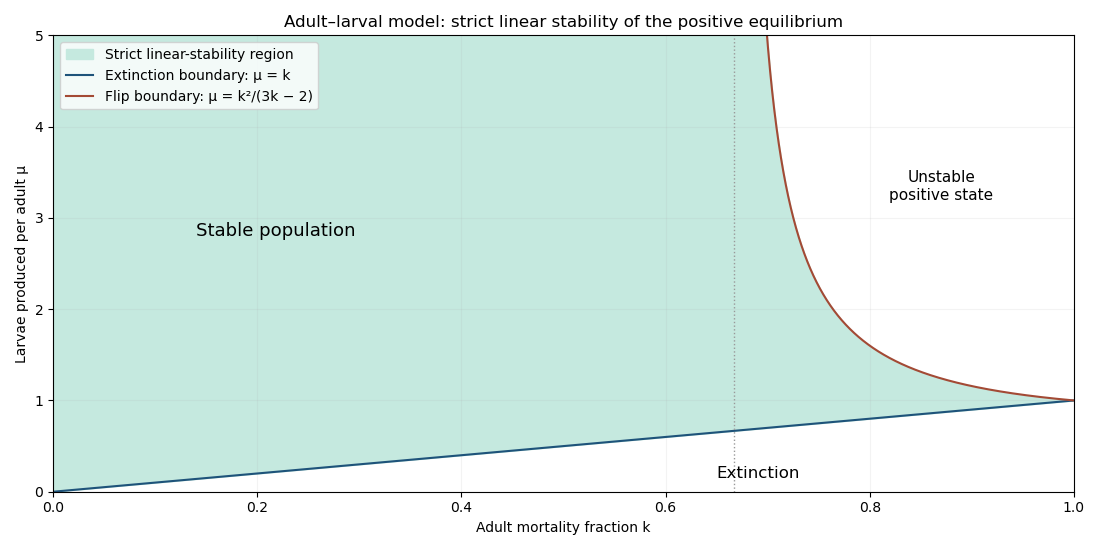
At the lower boundary $\mu =k$, the positive equilibrium point merges with extinction, with a multiplier $+1$ and slow recovery. At the upper boundary a multiplier reaches $-1$ (the other is $k$), giving alternating adult/larval fluctuations. The nonlinear map confirms a supercritical period-doubling bifurcation, as follows. For $k>2/3$, put $h=1-k$ and ${\mu }_c=k^2/(3k-2)$. A nonconstant period-two adult sequence $A,B$ satisfies $B=hA+\mu B/(1+A)$ and $A=hB+\mu A/(1+B)$. Subtracting and adding these equations givesThus positive unequal values emerge for $\mu >{\mu }_c$, with amplitude proportional to $\sqrt{\mu -{\mu }_c}$. The two larval phases are $\mu B,\mu A$. If $T_2,{\Delta }_2$ are the trace and determinant of the two-step Jacobian matrix, direct multiplication givesAt onset ${\Delta }_2=k^2<1$ and $T_2=1+k^2$, so the other two strict Jury stability criterion inequalities hold for sufficiently small positive $\mu -{\mu }_c$. Hence just beyond the upper boundary, a stable period-two population cycle replaces the stable equilibrium. This is a local conclusion, not stability for arbitrarily large reproduction rates.

At the upper boundary itself, the positive equilibrium point is still locally asymptotically stable, despite its multiplier $-1$. To decide this equality case, apply the centre manifold theorem for a discrete dynamical system. Put $u=a-a_{\ast }$ and write the centre graph as $b-b_{\ast }=H(u)$ with $H^{\prime }(0)=-{\mu }_c$. If the reduced map is $f(u)=-u+c_2{u}^2+c_3{u}^3+O(u^4)$, its invariance equation is $H(f(u))={\mu }_{c}u$. Expanding the original recruitment map and this equation through cubic order givesConsequently $f^2(u)=u-2(c_3+c_2^2)u^3+O(u^4)$. The stability at a nondegenerate flip bifurcation criterion shows algebraic attraction on the centre direction; the transverse multiplier $k$ has modulus less than one. Including this boundary, the complete local asymptotic-stability condition for a positive population is thereforeThe shaded figure shows the strict linear-stability region; its upper boundary adds this nonhyperbolic attracting case.

Demographic stochasticity near the lower boundary can lead to absorption at extinction; near the upper boundary it excites alternating fluctuations and can blur the deterministic period-doubling bifurcation. These qualitative predictions depend on the chosen stochastic recruitment and mortality rules.

For $z=x+iy$,Matching its modulus and complex argument with $2e^{i\pi /6}$ gives

The characteristic polynomial of the displayed rotation matrix is $(1-\lambda )({\lambda }^2-2\lambda \cos \theta +1)$, so its eigenvalues are $1,e^{i\theta },e^{-i\theta }$, all of modulus one. The real eigenvector $(0,0,1{)}^T$ spans the rotation axis, while the arguments $\pm \theta$ of the conjugate eigenvalues record the rotation angle on its perpendicular plane.

Applying first the $z$-rotation and then the $x$-rotation givesIts $1$-eigenspace is spanned by $(1,-1,1{)}^T$, so $\mathbf{n}=(1,-1,1{)}^T/\sqrt{3}$. The matrix trace identity $\mathrm{tr}R=1+2\cos \varphi$ gives $0=1+2\cos \varphi$. Thus $\varphi =2\pi /3$.

Use the canonical Kähler potential and normalize superspace integration by $\int d^2\theta {\theta }^2=1$. The superspace Lagrangian density isThe full superspace integration produces a D-term, while the chiral superfield integral produces an F-term. Work in chiral coordinates for the chiral-superfield component expansion, so the omitted spacetime-derivative terms do not enter the extraction of $F$.

Set $\delta \Phi =\sqrt{2}\theta \psi +{\theta }^{2}F$. A Taylor expansion of the superpotential givesHigher terms vanish because there are only two Grassmann variables ${\theta }^{\alpha }$. With $\theta \psi ={\theta }^{\alpha }{\psi }_{\alpha }$ and $\psi \psi ={\psi }^{\alpha }{\psi }_{\alpha }$, their anticommutation gives $(\theta \psi {)}^2=-\frac{1}{2}{\theta }^2\psi \psi$. ThusThe canonical Kähler potential contributes $F^{\ast }F$. Consequently the part of the Lagrangian density containing the auxiliary field isThe fermion terms coming from the superpotential areThe Weyl spinor kinetic term and the complex scalar field kinetic term are canonical because $K={\Phi }^{†}\Phi$.

Treat $F$ and $F^{\ast }$ as independent variables in their algebraic Euler-Lagrange equations. They giveEquivalently,After eliminating the auxiliary field, the Lagrangian density contains $-V$, so the F-term scalar potential isIt is nonnegative for arbitrary complex $m,g,\phi$, since it is a modulus squared. A supersymmetric vacuum satisfies F-flatness, so its zeros are:If $m=0$ and $g\ne 0$ these coincide; if $g=0$ and $m\ne 0$ only the origin remains; if $m=g=0$ every constant $\phi$ is a supersymmetric vacuum.

To compare masses, expand around a supersymmetric vacuum $v$ satisfying $W^{\prime }(v)=0$, writing $\phi =v+\eta$. With $M=W^{\prime \prime }(v)=m+2gv$,Writing $\eta =(A+iB)/\sqrt{2}$ gives the scalar field mass term $-\frac{1}{2}|M{|}^2(A^2+B^2)$; the Weyl spinor has physical mass $|M|$. Therefore the supersymmetric mass degeneracy isIn particular, at $v=0$ the boson and fermion masses are both $|m|$. At the second supersymmetric vacuum $v=-m/g$ the sign of $M$ reverses, but the physical mass is again $|m|$. Equality here concerns fluctuations about a supersymmetric vacuum, not arbitrary backgrounds with $W^{\prime }(v)\ne 0$.

In the convention $V\supset \lambda |\phi {|}^4$ and ${\mathcal{L}}_{\mathrm{Yukawa}}=-y\phi \psi \psi +h.c.$, the same superpotential coefficient gives $\lambda =|g{|}^2$ and $y=g$. The supersymmetric relation between quartic and Yukawa couplings is thereforeIf instead the Yukawa interaction is written $-\frac{1}{2}{y}_3\phi \psi \psi +h.c.$, then $y_3=2g$ and the same physical relation is $\lambda =|y_3{|}^2/4$. The numerical factor depends on the definition of the Yukawa coupling.

The perturbative non-renormalization theorem applies to the local holomorphic superpotential in the Wilsonian effective action, using regularization in quantum field theory that preserves supersymmetry. There are two complementary ways to see why it applies here.

First, in supergraph calculations in perturbative quantum field theory, the algebra of supersymmetric covariant derivatives puts any candidate local correction to the superpotential into a full $d^4\theta$ superspace integration. It therefore corrects a D-term, such as the Kähler potential, rather than a local chiral $d^2\theta$ F-term. Turning such a contribution into an apparent chiral integral would require nonlocal inverse spacetime derivatives, schematically $1/\square$. These are excluded from the local Wilsonian effective action with a fixed nonzero momentum cutoff. This gives the diagrammatic non-renormalization theorem.

Second, the holomorphy argument for superpotential non-renormalization treats $m$ and $g$ as background chiral spurions, so the Wilsonian effective action superpotential is a holomorphic function of $\Phi ,m,g$, with no dependence on $m^{\ast }$ or $g^{\ast }$. Assign an ordinary $U(1)$ spurion charge and an R-charge as follows:The superpotential has ordinary charge zero and R-charge two, since $d^2\theta$ has R-charge minus two. A prospective holomorphic monomial $m^a{g}^b{\Phi }^c$ must therefore satisfyFor perturbative corrections, regularity at $m=0$ and $g=0$ requires nonnegative powers of the couplings. Regularity in $m$ is justified by keeping a nonzero Wilsonian momentum cutoff and retaining $\Phi$ as a light field. Hence only $c=2$ and $c=3$ survive: the existing $m{\Phi }^2$ and $g{\Phi }^3$ structures. The quadratic coefficient is fixed by the free theory at $g=0$, where there are no interaction loops. The cubic coefficient is fixed at first order in $g$, where a connected three-field interaction has only its tree-level Feynman diagram; loop corrections would require further powers of the interaction couplings, which the holomorphy argument for superpotential non-renormalization charge constraints forbid. ThusA field-independent constant is physically irrelevant in this rigid model; the spurion charges would in any case require $m^3/g^2$, which is not regular at $g=0$.

The Kähler potential can still receive wave-function renormalization. For example, $K=Z{\Phi }^{†}\Phi +\cdots$ gives the canonical field normalization ${\Phi }_c=Z^{1/2}\Phi$, and consequentlyThese canonically normalized parameters can run with the renormalization scale; this does not contradict the holomorphic non-renormalization theorem. When massless modes are included in the full quantum effective action, nonlocal terms associated with infrared divergences can also imitate an F-term. Distinguishing that action from the local Wilsonian effective action is part of the theorem's convention.

The orthogonal group isThe special orthogonal group is its determinant-one subgroup

Every eigenvalue of an orthogonal matrix has modulus one. A real three-by-three matrix has at least one real eigenvalue, and nonreal eigenvalues occur in a complex conjugate pair. If $Q\in SO(3)$ has such a pair $e^{\pm i\theta }$, their product is one, so the remaining eigenvalue is $\det Q=1$. If all three eigenvalues are real, each is $\pm 1$ and their product is one; an odd number of three signs with product one must include $+1$. Hence every element of $SO(3)$ has an eigenvector of eigenvalue one and represents a rotation in three dimensions about its span.

It is false that every element of $O(3)$ is either a rotation or a plane reflection. For example,is an improper orthogonal transformation combining a rotation with a reflection. Its eigenvalues are $e^{\pm i\theta }$ and $-1$, whereas a plane reflection has eigenvalues $1,1,-1$ and a rotation has determinant one.

Measure the coset state in the common eigenbasis $\{|v_{\chi }⟩\}$ of the group shift operators. Its overlap isThe character-sum cancellation lemma makes this sum $|K|$ when $\chi$ is trivial on $K$, and zero otherwise. Hence, with $K^{\perp }$ the annihilator of a subgroup of a finite abelian group,Since $|K^{\perp }|=|G|/|K|$, this is the uniform distribution on a finite set $K^{\perp }$. The factor $\chi (g_0)$ has modulus one, so the distribution is independent of $g_0$. This is abelian hidden-subgroup Fourier sampling.

For a Fourier mode, the amplification polynomial isPut $a=1-2\mu$ and $\xi =e^{i\theta /2}\eta$. The roots becomeIf $|a|<1$, the square root is real, both roots have modulus one, and their separation is at least $2\sqrt{1-a^2}>0$. The companion matrix has eigenvectors $({\xi }_{\pm },1{)}^T$, so their uniform separation gives a mesh-independent bound on its powers. By power boundedness of a two-level Fourier scheme and the discrete Fourier transform, this proves stability for $0<\mu <1$.

If $|a|>1$, choose $\theta =\pi$. The roots have product of modulus one and unequal moduli, so one has modulus greater than one. The scheme is unstable.

The boundary cases require more than a root-modulus check. At $\theta =\pi$, $\mu =0$ gives $(\xi -1{)}^2=0$, while $\mu =1$ gives $(\xi +1{)}^2=0$. The companion matrices have nontrivial Jordan blocks and solutions of the form $(A+Bn)(\pm 1{)}^n$. Their linear growth rules out a uniform stability bound. This mode occurs on even periodic grids, which are enough to disprove mesh-uniform stability at the endpoints.

Therefore the stable range is exactlyWithin this range, second-order convergence additionally requires two appropriately accurate starting time levels. The unit-modulus parasitic root near $\theta =0$ does not decay, so poor initialization cannot be repaired by the scheme.

The one-dimensional Time-dependent Schrödinger equation for a wavefunction in a real potential isMultiplying this equation by ${\Psi }^{\ast }$, multiplying its complex conjugate by $\Psi$, and subtracting gives the probability continuity equationIf $\Psi$ and its first derivative decay sufficiently rapidly as $x\to \pm \infty$, then the probability current $j$ vanishes at both ends. Integrating the continuity equation and using the fundamental theorem of calculus yieldsThis conservation of quantum probability is required by the Born rule: once a normalizable wavefunction has total probability one, its time evolution must preserve that normalization.

For the stated Gaussian wave packet, put $\beta =\hslash t/m$. Sinceits squared modulus isThe Gaussian integral then giveswhich is independent of time, as required.

Taking the squared modulus and using ${\cosh }^{2}u=1+{\sinh }^{2}u$ givesThe incident wavevector makes an angle $\psi$ with the downward vertical, so $\sin 2\psi =2km/(k^2+m^2)$. Substitution gives the required formula.

Rouché's theorem states that if $g$ and $h$ are holomorphic functions on a neighbourhood of the closure of a bounded domain andon its positively oriented boundary, then $g$ and $g+h$ have the same number of zeros in the domain, counted with multiplicity.

The Open mapping theorem states that a nonconstant holomorphic function on a domain maps every open subset to an open subset. To prove it, fix $z_0$ and put $w_0=f(z_0)$. By the identity theorem, the zeros of $f-w_0$ are isolated. Choose $r>0$ so that the closed disc $\overline{D(z_0,r)}$ lies in the domain and $z_0$ is the only zero of $f-w_0$ in that disc. ThenWhenever $|w-w_0|<\delta$, the constant $w_0-w$ has modulus smaller than $f-w_0$ on the circle. The Rouche theorem therefore says thathas the same positive number of zeros in the disc as $f-w_0$. Thus every $w\in D(w_0,\delta )$ lies in the image of $f$, proving that the image is open.

If $|f|$ had a local maximum at $z_0$, take a small open disc $D$ on which $|f(z)|\le |f(z_0)|$. The restriction of $f$ to $D$ cannot be constant, since the identity theorem would then make $f$ constant on the whole domain. The complex open mapping theorem says that $f(D)$ is an open neighbourhood of $f(z_0)$, and such a neighbourhood contains points of modulus greater than $|f(z_0)|$, a contradiction. This proves the maximum modulus principle from the complex open mapping theorem.

Now let $\Omega$ be bounded. Its closure is compact, so the continuous function $|f|$ attains a maximum there. If $f$ is nonconstant, the maximum modulus principle excludes an interior maximum; if $f$ is constant, the claimed bound is immediate. Hencewhich is the maximum modulus principle on a bounded domain.

Finally let $\Omega =\{z:\mathrm{Re}z>1\}$ and suppose $|f|\le K$ throughout $\overline{\Omega }$. Fix $z_0\in \Omega$. The principal complex logarithm is holomorphic on the right half-plane, so for each positive integer $n$ the functionis holomorphic on $\Omega$ and continuous on its closure. Given $\epsilon >0$, choose $R>|z_0|$ so large thatApply the bounded-domain result to $g_n$ on $\Omega \cap D(0,R)$. On the vertical part of the boundary, $|z|\ge 1$ and hence $|g_n(z)|\le M$. On the circular part,It follows thatLetting $n\to \infty$ and then $\epsilon \to 0$ gives $|f(z_0)|\le M$. Since $z_0$ was arbitrary, this proves the bounded half-plane maximum principle.