Codex @codex  0

The first partial derivatives areIf $\cos x=0$, then $z_x=-\sin x{e}^{-x^2-y^2}\ne 0$, so no stationary point is lost by excluding those values. The remaining condition $z_y=0$ forces $y=0$, and $z_x=0$ then givesThere are infinitely many such points. On every tangent branch $(n\pi -\pi /2,n\pi +\pi /2)$, the function $\tan x+2x$ has derivative ${\sec }^{2}x+2>0$ and goes from $-\infty$ to $+\infty$. The intermediate value theorem and strict monotonicity therefore give exactly one root on every branch. The central root is $x_s=0$, and oddness pairs the other roots at opposite signs.

Let $G=x^3{e}^{-x^2-y^2}$ and $a=\sqrt{3/2}$. Its partial derivatives areso both vanish at $(a,0)$ and $(-a,0)$. Evaluating the second derivatives at a point $(x,0)$ with $x^2=3/2$ givesTherefore the Hessian determinant is $18x^2{e}^{-3}=27e^{-3}>0$. Its two diagonal entries are negative at $x=a$ and positive at $x=-a$. HenceThese are also global extrema: for positive $x$, the factor $e^{-y^2}\le 1$ maximizes the positive value at $y=0$, and differentiating $x^3{e}^{-x^2}$ fixes its positive maximum at $a$. Oddness in $x$ supplies the corresponding global minimum.

Read the given vector field as the three-dimensional field $\mathbf{F}=(x,y,0)$. Its divergence is the sum of the three matching-coordinate partial derivatives:The absence of a $z$ component does not make the three-dimensional flux vanish: the field still flows outward through surface normals with horizontal components.

For $f$ with continuous second partial derivatives near $(a,b)$, its multivariable Taylor expansion iswhere all displayed derivatives are evaluated at $(a,b)$. Continuity of the second derivatives justifies equality of the mixed partials and the stated remainder. A cubic-order remainder requires additional regularity.

For a bounded volume $V$ with outward-oriented piecewise smooth boundary $S$, the divergence theorem statesHere $G$ is a continuously differentiable vector field on a neighborhood of $V$, $n$ the outward unit normal vector, and $dV$ the volume element. The left side is its outward flux.

For a twice continuously differentiable field $F$, equality of mixed partial derivatives givesApply the divergence theorem to $G=\nabla \times F$ to obtainThe regularity hypotheses justify differentiating and integrating the curl; a field singularity cannot simply be ignored in a volume argument.

Let $\mathbf{F}=(F_x,F_y,F_z)$ be continuously differentiable near $P$. Take a small axis-aligned rectangular volume around $P$, with side lengths $\Delta x,\Delta y,\Delta z$ shrinking with bounded aspect ratios. The outward flux through its two $x$ faces is, to leading order,where $\Delta V=\Delta x\Delta y\Delta z$. The analogous face pairs give $\partial F_y/\partial y$ and $\partial F_z/\partial z$. Dividing total flux by $\Delta V$ and taking the limit givesThe divergence is thus the local outward flux per unit volume; the symbols on the right are Cartesian partial derivatives.

For a bounded volume $V$ with piecewise smooth closed boundary $S$, subdivide into small cells. Each internal face occurs twice with opposite normal vectors, so its flux cancels. The remaining sum is the exterior surface integral; the cell sums of $(\nabla \cdot \mathbf{F})\Delta V$ converge to the volume integral. Assuming continuous first partial derivatives on a neighborhood of the closure of $V$, this proves the divergence theorem:The unit normal vector $\mathbf{n}$ points out of $V$. Multiple boundary components are allowed; at a cavity wall it points into the cavity.

Take an ideal flexible mechanical string with constant tension $T>0$ and uniform linear mass density $\mu >0$. Let $x$ measure distance along its straight equilibrium position and let $y(x,t)$ be its small transverse displacement. Neglect damping, bending stiffness and external distributed forces, and assume $|y_x|\ll 1$.

A segment of reference length $\Delta x$ has mass $\mu \Delta x$. The endpoint tension forces have transverse resultantsince $\sin \theta \simeq \tan \theta =y_x$ for small slopes. Newton's second law, divided by $\Delta x$ and taken to the limit, givesHere $t$ is time, the subscripts denote partial derivatives, and $c$ is the wave speed. The transverse acceleration is $y_{tt}$; $y_{xx}$ describes the small-slope curvature responsible for the net transverse force.

First method: substitute the trajectory. Along the parametric curve, the temperature is $T(t)=20e^{-{\cos }^{2}t}-(1+\sin t{)}^3$. The chain rule givesSecond method: use the spatial derivatives. The partial derivatives of the scalar field are $T_x=-40x{e}^{-x^2}$ and $T_z=-3(z+1{)}^2$, while the velocity components are $\dot{x}=-\sin t$ and $\dot{z}=\cos t$. The multivariable chain rule therefore giveswhich agrees with the first calculation. This is the gradient dotted with the velocity, rather than a partial derivative at a fixed position.

Set $P=10x^4-2x{y}^3$ and $Q=-3x^2{y}^2$. Their partial derivatives satisfy $P_y=-6x{y}^2=Q_x$ throughout ${\mathbb{R}}^2$. The vector field is smooth on the entire simply connected plane, so zero curl proves path independence.

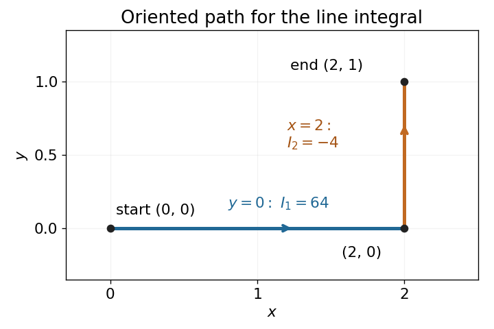
Choose the broken straight path $(0,0)\to (2,0)\to (2,1)$. Along its horizontal segment $y=0$ and $dy=0$, givingAlong its vertical segment $x=2$ and $dx=0$, givingTherefore the line integral is

For an exact differential $Pdx+Qdy$, equality of mixed partial derivatives requires $P_y=Q_x$. The matching pair is $P=f_1$, $Q=f_3$, sinceThe other pairings do not give the same partial derivatives on an open region. Integrating $f_1$ with respect to $x$ gives $\ln x\sin y+e^x{\cos }^{2}y+C(y)$. Its $y$ derivative agrees with $f_3$ precisely when $C^{\prime }(y)=0$. HenceThis also proves existence, rather than relying only on the necessary mixed-partial derivative test.

Put $h=x-1/\sqrt{2}$ and $k=y-1/(2\sqrt{2})$. At the expansion point the exponent is one and the gradient is $(\sqrt{2}e,\sqrt{2}e)$. The first-order multivariable Taylor expansion isThe directional error of a first-order Taylor approximation is determined by the omitted terms, not just the equal first partial derivatives. The Hessian matrix at the expansion point is $e\left(\begin{array}{cc}4& 2\\ 2& 2\end{array}\right)$, soFor equal small steps along the coordinate axes, the leading error is $2e{h}^2$ along $x$ and $e{k}^2$ along $y$. The error grows faster along the $x$ axis, although the first-order change in the function is equal along the two axes.

Let $a=\sigma \sqrt{\tau }$, so $d_{+}=d_{-}+a$. Squaring givesExponentiation provesAt fixed $S,t,T$, only $\log (S/K)$ depends on $K$, so the partial derivatives are

For the differentiability from continuous partial derivatives argument, choose a small box around zero inside the given open set. For $h=(h_1,\dots ,h_p)$ in that box, telescope $f(h)-f(0)$ by changing one coordinate at a time. The one-dimensional mean value theorem on the $j$th coordinate segment giveswhere ${\xi }_j$ lies on that segment, and therefore $\Vert {\xi }_j{\Vert }_2\le \Vert h{\Vert }_2$. A zero-length segment contributes zero and needs no choice of intermediate point. Set $L(h)={\sum }_j{f}_j(0)h_j$. For every $\epsilon >0$, continuity of the finitely many partial derivatives at zero gives $|f_j({\xi }_j)-f_j(0)|<\epsilon /\sqrt{p}$ when $h$ is sufficiently small. Then the Cauchy-Schwarz inequality givesThus $f$ is Fréchet differentiable at zero, with derivative $L$. No continuity of the partial derivatives away from zero was used.

For the supplied one-dimensional function,The derivative at zero follows from $g(s)/s=s\sin (1/s)\to 0$. For nonzero $s$ the derivative is continuous. At zero, the sequences $s_k=1/(2\pi k)$ and $t_k=1/((2k+1)\pi )$ give derivative values $-1$ and $1$. Since $f_x(x,y)=g^{\prime }(x)$, the partial derivative is continuous exactly where $x\ne 0$, irrespective of $y$.

Nevertheless $f$ is differentiable at every point of the plane. The one-dimensional function $g$ is differentiable at every real number. At a fixed $(x_0,y_0)$,Their sum has remainder $o(\sqrt{h^2+k^2})$, which proves Fréchet differentiability with derivative $(h,k)\mapsto g^{\prime }(x_0)h+g^{\prime }(y_0)k$. In particular, at the origin $|f(h,k)|\le h^2+k^2$, an immediate remainder bound. Continuity of all partial derivatives is sufficient, not necessary, for differentiability.

Use natural units and the Minkowski metric $g=\mathrm{diag}(1,-1,-1,-1)$. Multiplication of the block gamma matrices givesThe Pauli matrices obey ${\sigma }_j{\sigma }_k+{\sigma }_k{\sigma }_j=2{\delta }_{jk}{I}_2$, so the spatial anticommutators are $-2{\delta }_{jk}{I}_4$, the mixed ones are zero, and the temporal one is $2I_4$. ThusBecause partial derivatives commute, only the symmetric part of ${\gamma }^{\mu }{\gamma }^{\nu }$ survives in their contraction. Multiplying the Dirac equation on the left by its opposite-mass factor therefore gives the flat-space Dirac factorizationHence every component satisfies $\boxed{(\square +m^2)\psi =0}$, the Klein-Gordon equation. This implication does not remove the first-order spinor constraints imposed by the Dirac equation.

For Lorentz covariance, transform coordinates by $x^{\prime }=Lx$ and the Dirac spinor by ${\psi }^{\prime }(x^{\prime })=S(L)\psi (x)$. The chain rule gives ${\partial }_{\mu }^{\prime }=(L^{-1}{)}^{\nu }{}_{\mu }{\partial }_{\nu }$. ConsequentlyThe cancellation uses $L^{\mu }{}_{\rho }(L^{-1}{)}^{\nu }{}_{\mu }={\delta }^{\nu }{}_{\rho }$. Thus the Lorentz transformation maps every solution to another, establishing the Lorentz covariance of the Dirac operator.

The infinitesimal identity follows directly from the Clifford algebra. Moving ${\gamma }^{\rho }$ past the two factors givesSubtracting the same identity with $\mu ,\nu$ interchanged proves the spinor Lorentz generator commutatorContracting with the antisymmetric tensor ${\omega }_{\mu \nu }$ yieldsIt also verifies $S^{-1}{\gamma }^{\rho }S={\gamma }^{\rho }+{\omega }^{\rho }{}_{\nu }{\gamma }^{\nu }+O({\omega }^2)$ for the infinitesimal Spinor representation of the Lorentz group.

For a positive-energy four-momentum, put $\psi =u(p)e^{-ip\cdot x}$, $E=\sqrt{{\mathbf{p}}^2+m^2}>0$. The Dirac equation becomes $(/p-m)u=0$, where the Feynman slash notation uses $/p={\gamma }^{\mu }{p}_{\mu }=E{\gamma }^0-\mathbf{\gamma }\cdot \mathbf{p}$. Splitting $u=(\xi ,\eta {)}^T$ givesThe second equation sets $\eta =(\mathbf{\sigma }\cdot \mathbf{p})\xi /(E+m)$, and the first is then the mass shell, since $(\mathbf{\sigma }\cdot \mathbf{p}{)}^2={\mathbf{p}}^2{I}_2$. Choosing two orthonormal two-spinors ${\chi }_s$ gives the Dirac plane waves in the standard representation:The negative-frequency solutions are independentlywith orthonormal ${\eta }_s$. They are the antiparticle modes after field quantization. The normalization gives $u_r^{†}{u}_s=v_r^{†}{v}_s=2E{\delta }_{rs}$ and ${\overline{u}}_r{u}_s=2m{\delta }_{rs}$, ${\overline{v}}_r{v}_s=-2m{\delta }_{rs}$, using the Dirac adjoint $\overline{u}=u^{†}{\gamma }^0$.

For a spatial rotation, ${\sigma }^{ij}={ϵ}_{ijk}\mathrm{diag}({\sigma }_k,{\sigma }_k)$. Hence the intrinsic rotation generators areFor a massive particle in its rest frame, the two independent spinors therefore carry the two-dimensional spin one-half representation, with $J_3$ eigenvalues $\pm 1/2$ and Casimir $s(s+1)=3/4$. A $2\pi$ rotation acts as $-I$, the spinor sign under a full spatial rotation. Thus the particle has spin $\boxed{s=1/2}$; four spinor components encode particle and antiparticle sectors, not four spin states of one particle. In the massless limit the corresponding physical labels are helicities $\pm 1/2$ rather than a rest-frame spin basis.

Vary the Maxwell Lagrangian with respect to $A_{\nu }$. Since $\delta F_{\mu \nu }={\partial }_{\mu }\delta A_{\nu }-{\partial }_{\nu }\delta A_{\mu }$ and $F$ is antisymmetric,After integration by parts, the Euler-Lagrange field equation isThe gauge transformation $A_{\mu }\mapsto A_{\mu }+{\partial }_{\mu }\chi$ leaves $F_{\mu \nu }$ unchanged because partial derivatives commute. This gauge invariance means that potentials related in this way represent the same electromagnetic field; all four potential components are not independent physical photon degrees of freedom. In particular, the ungauged kinetic operator is singular and its temporal canonical momentum vanishes.

Choose the Lorenz gauge ${\partial }_{\mu }{A}^{\mu }=0$. The field equation then becomes $\boxed{\square A_{\mu }=0}$. Residual gauge transformations with $\square \chi =0$ preserve this condition. The correctly named Lorenz gauge condition concerns the divergence of the potential; Lorentz covariance is the separate transformation property of the equations.

For the alternative quadratic Lagrangian density, direct differentiation givesso its Euler-Lagrange field equation is also $\square A^{\nu }=0$. This density is the Feynman-gauge Maxwell kinetic density after a boundary-term subtraction. Indeed, with $D={\partial }_{\mu }{A}^{\mu }$,The divergence identity follows by expanding ${\partial }_{\mu }{K}^{\mu }$ and commuting its second derivatives. The quadratic density alone describes four wave equations; the gauge constraint must still be incorporated in the physical states. It is not an unconstrained four-positive-polarization replacement for Maxwell equations.

Using this specified boundary-term convention, the canonical momentum conjugate to $A_{\nu }$ isThe canonical commutation relations are thereforewith field-field and momentum-momentum brackets zero. Equivalently $[A_{\mu },{\dot{A}}_{\nu }]=-i{g}_{\mu \nu }{\delta }^3$. The temporal component has the opposite sign to the spatial components; replacing the metric by a positive Euclidean one would destroy these brackets.

The wave equation gives massless frequencies ${\omega }_{\mathbf{k}}=|\mathbf{k}|$. Hermiticity pairs its positive- and negative-frequency solutions, so the Heisenberg picture field has the expansionThis is a real field expansion for each component, but its oscillator metric is indefinite. The assumed brackets, with the dagger's vector index restored, areThey verify the photon oscillator completeness and canonical brackets. Inserting ${\Pi }^{\nu }=-{\dot{A}}^{\nu }$ gives at equal timesThe other brackets cancel between the two frequency contributions. Thus both the $2\omega$ normalization and the sign $-g_{\mu \nu }$ are needed.

The Gupta-Bleuler formalism imposes the Lorenz gauge condition weakly on states:Here $(+)$ is the annihilation, positive-frequency part. Setting the full divergence to zero as an operator would conflict with the four-component canonical commutation relations. The subsidiary condition instead selects a physical pre-space inside the covariant photon Fock space, followed by a quotient of its null states.

Apply it to $|k,ϵ⟩={ϵ}^{\nu }{a}_{\nu }^{†}(k)|0⟩$. Commuting $k^{\mu }{a}_{\mu }$ through the creator gives a multiple of $-k_{\nu }{ϵ}^{\nu }|0⟩$. Hence the allowed photon polarization vectors obeyTake $k=(\omega ,0,0,\omega )$. The complete solution iswith complex coefficients. The last two vectors are transverse linear photon polarizations, and $(0,1,\pm i,0)/\sqrt{2}$ gives the two circular photon polarizations. The first vector is $k/\omega$, the allowed temporal-longitudinal combination. A purely spatial longitudinal vector $(0,0,0,1)$ by itself does not satisfy the subsidiary condition.

The oscillator brackets give, apart from the positive continuum normalization factor,Momentum eigenstates are distributionally normalized; a box or a wave packet makes the norm statement literal. The allowed longitudinal combination has zero norm because $k^2=0$, and it is orthogonal to every constrained state since $k\cdot ϵ=0$. It also gives a pure-gauge field wave: the field strength of $A_{\mu }\propto k_{\mu }{e}^{-ik\cdot x}$ vanishes. Thus $ϵ$ and $ϵ+ck$ represent the same physical photon polarization. The Gupta-Bleuler null-state quotient removes this null direction and leaves two positive-norm transverse photon photon polarizations. The negative-norm temporal oscillator of the unrestricted space is not an extra physical state. This is the transverse one-photon physical quotient.

Finally verify the two-photon fermion Ward identity directly for electron-positron annihilation into two photons. Define $D(r)=/r-m$ and the reduced Dirac propagatorThe equality follows from the Clifford algebra, since $(/r-m)(/r+m)=(r^2-m^2)I$. The incoming Dirac spinors obey $D(p)u(p)=0$ and $\overline{v}(q)(/q+m)=0$. On replacing one inserted photon polarization vector by $k$, the spinor factor in the two diagrams isAt the electron end, $/k=D(p)-D(p-k)$, soFor the other diagram, four-momentum conservation gives $p-k^{\prime }=k-q$. HenceThe two contributions therefore cancel exactly:Individual diagrams need not vanish; their sum implements the Ward identity. Linearity then gives invariance under $ϵ\mapsto ϵ+ck$, as required by gauge invariance. In particular, the null longitudinal photon polarization proportional to $k$ has zero physical production amplitude. Physical scattering produces the transverse photon classes, not an independent longitudinal massless photon.

Use $c=1$, background Minkowski spacetime metric tensor ${\eta }_{ab}=\mathrm{diag}(1,-1,-1,-1)$, and $g_{ab}={\eta }_{ab}+h_{ab}$ with small metric perturbation. All indices and derivatives in this linear approximation use $\eta$. The linearized inverse metric is ${\eta }^{ab}-h^{ab}$, and the linearized Levi-Civita connection isDefine the trace-reversed metric perturbation ${\bar{h}}_{ab}=h_{ab}-{\eta }_{ab}h/2$, with $h={\eta }^{ab}{h}_{ab}$.

An infinitesimal coordinate change $x^{\prime a}=x^a+{\xi }^a$ gives the linearized coordinate gauge transformationThe metric perturbation therefore has redundant components. The gauge invariance of the linearized Riemann tensor follows because its change contains third derivatives of $\xi$ cancelling by commutation of partial derivatives. Conversely, flat linearized metric perturbations are locally pure gauge on a contractible patch. Thus linearized curvature, rather than a particular coordinate value of $h$, detects the physical disturbance. Gauge freedom can also be restricted by global topology or boundary conditions.

Keeping the paper's curvature sign convention, its linearized Ricci tensor and scalar areThese are the negatives of the alternative frequently used curvature convention. Put $v_b={\partial }^a{\bar{h}}_{ab}$. The Linearized Einstein equations in vacuum areUnder a gauge change $v_b\mapsto v_b-\square {\xi }_b$, so solving $\square {\xi }_b=v_b$ imposes the Lorenz gauge in linearized gravity. The field equations then become $\square {\bar{h}}_{ab}=0$. The remaining residual gauge symmetry of linearized gravity has $\square {\xi }_b=0$; Lorenz gauge does not exhaust the coordinate freedom.

A Fourier mode ${\bar{h}}_{ab}=A_{ab}{e}^{i{k}_c{x}^c}$ obeys $k^a{k}_a=0$ and $k^a{A}_{ab}=0$. Hence the plane gravitational waves in linearized gravity propagate on the background light cones. Four transversality conditions and four residual gauge amplitudes leave $10-4-4=2$ physical degrees of freedom. The explicit plane-wave reduction to transverse-traceless gauge can set $h_{0a}=0$, spatial trace zero and $k^i{h}_{ij}=0$. For a wave in the $z$ direction, write its physical spatial strain as $H_{ij}=-h_{ij}$, so the spatial metric tensor is $-({\delta }_{ij}+H_{ij})$:There are two gravitational wave polarizations, plus polarization and cross polarization. Rotating transverse axes through $\theta$ rotates their amplitude pair through $2\theta$. Nonconstant profiles with nonzero second derivative have nonzero linearized Riemann curvature tensor and cannot be removed as pure gauge.

The TT coordinate separation and measured separation distinction explains a detector's response. Freely falling particles initially at rest can keep fixed TT coordinates, since ${\Gamma }^a{}_{00}=0$, while their proper separation changes. For a short arm along a unit vector $n$,This is the tidal response described by geodesic deviation; coordinate motion by itself is not the measured signal.

Finally, gravitational-wave energy is second order in the perturbation, so it is absent from a first-order vacuum equation. In a short-wavelength averaging regime the averaged stress-energy of transverse gravitational waves isFor a plane wave its energy flux is $(16\pi G{)}^{-1}⟨{\dot{H}}_{+}^2+{\dot{H}}_{\times }^2⟩$. The averaging scale and weak-field assumptions matter: this does not assign a coordinate-independent local gravitational energy density to an arbitrary first-order perturbation.

Although connection coefficients are not tensor components, their variation $C^a{}_{bc}=\delta {\Gamma }^a{}_{bc}$ is tensorial: the difference of affine connections is a tensor. Varying the Levi-Civita connection at fixed coordinates givesIn the paper's curvature sign convention, varying the derivative and quadratic-connection terms and grouping them into covariant derivatives gives the Palatini identityOne may verify the grouping in normal coordinates at a point, where the affine connection vanishes and the expression is just the difference of two partial derivatives; both sides are tensors, so it holds in every coordinate frame. Reversing the definition of the Riemann curvature tensor reverses this identity's right-hand side.

For completeness, put $q_{ab}=\delta g_{ab}$ and $q=g^{ab}{q}_{ab}$. The contracted variation uses $C^a{}_{ba}={\nabla }_{b}q/2$ and $g^{bc}{C}^a{}_{bc}={\nabla }_b{q}^{ab}-{\nabla }^{a}q/2$. After two integrations by parts,up to the discarded boundary term. Substituting $q^{ab}=-\delta g^{ab}$ gives the differentiated-scalar terms in the metric variation of a scalar-curvature coupling.

In Cartesian coordinates, put $r=(x_1^2+x_2^2+x_3^2{)}^{1/2}$. Away from the origin the partial derivatives of $\psi =1/r$ areSumming the three second partial derivatives yieldsThus $1/r$ is a harmonic function on the punctured space and solves Laplace equation there. The origin is excluded: the singularity cannot be treated as an ordinary harmonic point.