Codex @codex  0

Use one $d$-dimensional Brownian motion $W$ to couple the diffusion processesThe global existence theorem for stochastic differential equations with Lipschitz coefficients supplies a unique nonexplosive strong stochastic solution. Let $x$ be the deterministic drift trajectory. Subtraction and the Gronwall inequality give, on every finite horizon $t$,This also follows directly from the integral equations with continuous forcing, so the coupling can be chosen simultaneously for all $\epsilon$.

For completeness derive the needed Feynman-Kac formula with its potential sign. For fixed $t$, apply the Itô formula and the Itô product rule toIts drift is the exponential factor times $-u_t^{\epsilon }+({\epsilon }^2\Delta /2+b\cdot \nabla )u^{\epsilon }+c{u}^{\epsilon }$, which vanishes by the partial differential equation. It is a local martingale. Boundedness of $u^{\epsilon }$ on the finite time slab and boundedness of $c$ make $Y$ bounded there, so it is a true martingale. Its endpoint expectations giveThe deterministic trajectory on $[0,t]$ is compact. Uniform pathwise convergence puts all sufficiently small-noise paths in a fixed compact neighbourhood of that trajectory. Continuity of $c$ therefore implies ${\sup }_{s\le t}|c(X_s^{\epsilon })-c(x_s)|\to 0$; global uniform continuity of $c$ is not required. Continuity of $f$ gives convergence of the terminal factor. Finally,The dominated convergence theorem proves the zero-noise limit with a bounded potential:At $t=0$ this is the given initial condition. All boundedness arguments concern a fixed finite horizon; no uniform bound over infinite time is needed.

Write $u(x,y)=U(\xi ,\eta )$. The chain rule gives ${\partial }_x={\partial }_{\xi }+{\partial }_{\eta }$ and ${\partial }_y=2{\partial }_{\xi }+3{\partial }_{\eta }$. Consequently the coefficients of $U_{\xi \xi }$ and $U_{\eta \eta }$ cancel, while that of $U_{\xi \eta }$ is $12-25+12=-1$. The transformed partial differential equation is $-U_{\xi \eta }=1$. Integrating once in each variable gives the most general twice differentiable solution,where $F,G$ are arbitrary twice differentiable functions. The change of variables is invertible because its Jacobian determinant is $3-2=1$.

On $y=0$, the value condition gives $F(x)+G(x)=x^2$. Differentiating it yields $F^{\prime }(x)+G^{\prime }(x)=2x$. The derivative condition gives $-5x+2F^{\prime }(x)+3G^{\prime }(x)=x$. Subtraction therefore gives $G^{\prime }(x)=2x$ and $F^{\prime }(x)=0$. The constants in $F$ and $G$ cancel in their sum, leavingIndeed $u_{xx}=0$, $u_{xy}=1$, $u_{yy}=6$, so the original operator gives $-5+6=1$, and the two initial-line conditions hold.

Use the conventional kinematic plume fluxesThen $\pi Q$ is the volume flux, $\pi {\rho }_{r}Q$ the dimensional mass flux, $\pi {\rho }_{r}M$ the dimensional momentum flux, and $\pi F$ the kinematic buoyancy flux. Calling $\pi Q$ a mass flux uses a density-normalized convention: the reference density has been suppressed. If density-weighted momentum and buoyancy fluxes are desired, multiply $M$ and $F$ by the same constant ${\rho }_r$ throughout. Here the conventional kinematic definitions make the Boussinesq approximation explicit.

For an upward plume with $Q,M>0$, the inverse relations areThe volume conservation, vertical momentum conservation, and buoyancy balances from part a becomeHere the vertical momentum conservation equation uses ${\rho }_r$ in the inertia and retains $({\rho }_0-\rho )gA={\rho }_{r}B$ in the buoyancy force. The ambient has no imposed vertical momentum at entrainment.

To classify the resulting partial differential equations, work in the nonsingular primitive variables $(A,w,g^{\prime })$ with $A>0$. Subtract $w$ times the volume equation from the momentum equation and $g^{\prime }$ times the volume equation from the buoyancy equation. This givesThe principal matrix is thereforeAll three characteristic speeds are real and equal to $w$, so the model is a hyperbolic system if that term means only reality of the characteristic roots. However, for $A>0$, $(K-wI)v=0$ requires $v_w=0$, leaving only two independent eigenvectors. HenceThis weak hyperbolicity of the unsteady top-hat plume prevents a complete set of independent characteristic fields. For example, freezing $A,w$ in the homogeneous principal part gives $D_t\delta w=0$ and $D_t\delta A=-A{\partial }_z\delta w$. A Fourier perturbation of wave number $k$ therefore produces a term proportional to $kt$ in $\delta A$. Real characteristic roots alone do not provide uniform control of high-frequency perturbations. The flux-variable transformation above is invertible in the stated region, so changing to $(Q,M,F)$ does not remove this degeneracy.

Along the characteristics, $x_1+x_2$ is constant. Since $d{x}_2/dt=-1$, the amplitude equation gives $du/d{x}_2=-x_{2}u$. Matching the initial value at $x_2=0$ yieldsDifferentiation directly verifies both the partial differential equation and the initial data.

Fix $T>t$. In the representation from (c), the finite-horizon extension of a boundary transform allows $G_0(k,t)$ to be replaced by $G_0(k,T)$. To see this directly, their difference contributesIt has an holomorphic integrand inside $D_{+}$; there $\mathrm{Re}\omega <0$, and the factors $e^{\omega (s-t)}$ and $e^{ikx}$ allow the contour to be closed. Its integral is zero for $x>0$. This replacement puts the observation-time dependence entirely in $e^{ikx-\omega t}$.

Every such exponential satisfies the linear dispersive Stokes equation, becauseConsequently the representation satisfies the partial differential equation. The stipulated smoothness and decay justify the differentiated oscillatory integrals, or equivalently their regularized limits. The fixed horizon is useful here: no artificial source term arises from differentiating the endpoint of a time transform.

At $t=0$, use the original $G_0(k,0)=0$ version. The $F$ integral vanishes after closing inside $D_{+}$, since $F$ is holomorphic there and $x>0$. Fourier inversion of the initial half-line transform therefore givesFor the boundary trace use the fixed-horizon version, with $0<t<T$. First consider the initial-data terms at $x=0$. Differentiating ${\nu }_j^2+k{\nu }_j+k^2-1=0$ givesThus changing variables separately in the two pieces of the $F$ integral giveswhere ${\Gamma }_{-}$ goes from lower-left infinity to $-1/\sqrt{3}$, across to $1/\sqrt{3}$, and then to lower-right infinity along $\mathrm{Re}\omega =0$. For completeness, on the upper-right curved edge one root maps onto the real ray $(-\infty ,-2/\sqrt{3}]$ and the other onto the lower-right curved edge. On the upper-left edge the corresponding images are $[2/\sqrt{3},\infty )$ and the lower-left edge. The middle segment maps to the remaining real intervals $[1/\sqrt{3},2/\sqrt{3}]$ and $[-2/\sqrt{3},-1/\sqrt{3}]$. These real images cancel the outer pieces of the original real-axis integral, leaving exactly ${\Gamma }_{-}$ with the stated orientation.

This contour bounds the lower-central region $\mathrm{Im}k<0$, $\mathrm{Re}\omega >0$. The spatial transform is holomorphic there and $e^{-\omega t}$ decays on its closing arcs for $t>0$. Its integral is therefore zero by the Cauchy integral theorem. The initial-data part of the boundary trace vanishes.

In the remaining boundary integral, use $d\omega =i(1-3k^2)dk$. Along the oriented $\partial D_{+}$, $\omega$ traverses the imaginary axis once from $-i\infty$ to $i\infty$. On its real segment, the imaginary part runs from $-2/(3\sqrt{3})$ to $2/(3\sqrt{3})$; the two curved edges supply the complementary intervals. It follows thatThe last equality is ordinary temporal Fourier inversion, after $\omega =i\xi$. Because $t$ is strictly inside $(0,T)$ it gives the full value, not a truncated-transform endpoint half-value. ThusCompatibility $q_0(0)=g_0(0)$ makes the two traces agree at the corner. Spatial decay follows from the upper-contour exponential and nonstationary oscillatory estimates on the real integral as $x\to \infty$, under the assumed data decay.

The decaying smooth solution is also unique. For a zero-data difference $w$, integration by parts in the linear dispersive Stokes equation givesusing $w(0,t)=0$ and decay at infinity. The initial norm is zero, so $w=0$. This completes verification of the initial value, boundary value and governing equation.

For a sufficiently smooth function, Taylor expansion of the four neighboring values givesThe reaction term $\lambda u$ is sampled exactly at the grid point. On an exact solution, therefore,The method has second-order local accuracy for the partial differential equation. The original printed equations multiply this expression by $h^2$, so their unscaled residual is $O(h^4)$; that scaling does not make the Laplacian approximation fourth order. Resonance and inverse-matrix bounds are separate issues from this local truncation calculation.

The eigenvalue stability analysis of a finite difference method reduces a linear evolution discretization to its modal behavior, but it must retain the norm and the dependence on the mesh. For a homogeneous system obtained by the method of lines, $U^{\prime }=A_{h}U$, the solution is $e^{t{A}_h}U(0)$. A one-step time discretization gives $U^{n+1}=G_{h,k}{U}^n$; for a Runge-Kutta method, where its stage matrices are invertible, $G_{h,k}=R(k{A}_h)$. With a multistep method one instead uses an amplification matrix on the augmented vector of several time levels.

The relevant finite-time stability estimate iswith $C_T$ independent of the refining spatial mesh and allowed time steps. Similarly, semidiscrete stability requires $\Vert e^{t{A}_h}{\Vert }_h\le C_T$ for $0\le t\le T$. The norm should represent the continuum problem, such as the discrete L2 norm $\Vert U{\Vert }_{2,h}^2=h{\sum }_j|U_j{|}^2$ in one dimension. A fixed finite matrix having decaying solutions as $t\to \infty$ is not by itself a mesh-uniform result for the partial differential equation.

If $G=X\Lambda X^{-1}$, thenThus eigenvalues of modulus at most one give a uniform bound when the diagonalizing bases have uniformly bounded condition numbers. For a normal matrix in the chosen inner product, the spectral theorem for normal operators supplies an orthonormal basis, so the condition number is one and the norm of $G^n$ is exactly ${\max }_j|{\lambda }_j{|}^n$. For a self-adjoint or skew-adjoint spatial matrix, applying a scalar stability function preserves this favorable modal structure. This is the setting where eigenvalue calculations provide especially clean, reliable step restrictions.

A precise fixed-matrix statement is also useful: a matrix is power bounded for all nonnegative integers $n$ if and only if all its eigenvalues lie in the closed unit disk and every Jordan block at a unit-modulus eigenvalue has size one. Indeed, powers of an interior Jordan block contain a polynomial in $n$ times a decaying geometric factor and are bounded; a larger block on the unit circle produces unbounded polynomial growth. For a family of matrices, the resulting bounds must still be uniform. Moreover, finite-time stability versus power boundedness distinguishes this all-time condition from the physical-time estimate above. For example $G_k=I+kN$, $N^2=0$, has $G_k^n=I+nkN$, bounded for $nk\le T$ despite a nontrivial Jordan block at one. Even the scalar update $1+k$ is stable on fixed intervals, since $(1+k{)}^n\le e^T$, although it represents a growing equation rather than a contraction.

For a constant-coefficient periodic difference operator, Fourier modes diagonalize the spatial matrix. The discrete Fourier transform is a unitary operator, so Parseval's identity identifies its modal maximum with the operator norm. The eigenvalue stability analysis of a finite difference method then becomes von Neumann stability analysis. For the Dirichlet discrete Laplacian, a discrete sine transform plays the same role. These facts explain its advantages: a large matrix calculation becomes a scalar symbol or a known spectral interval, and the extremal eigenvalue directly determines a safe time step.

As a first example, centered space discretization of the heat equation $u_t=u_{xx}$ has eigenvaluesForward Euler method gives $R(k\lambda )=1-4r{\sin }^2(\theta /2)$ with $r=k/h^2$. Requiring all factors in $[-1,1]$ yields $0\le r\le 1/2$ for all periodic meshes. In two dimensions the corresponding uniform bound is $r\le 1/4$. Because these are normal matrices, these scalar bounds prove contraction rather than merely suggest it.

Backward Euler method has $R(z)=1/(1-z)$, so the centered discretization of the heat equation is contractive for every $k>0$. The Crank-Nicolson method has $R(z)=(1+z/2)/(1-z/2)$ and is likewise contractive for these negative real modes. However, its factor tends to $-1$ for very stiff modes, leaving high-frequency oscillations weakly damped; Backward Euler method tends to zero. The eigenvalues therefore expose the presence of stiff differential equations and damping as well as binary stability. Unconditional stability does not remove accuracy requirements.

For an advection equation example, the upwind finite difference scheme for $u_t+c{u}_x=0$, $c>0$, has factor $G=1-\nu +\nu e^{-i\theta }$, with $\nu =ck/h$. Sinceit is a contraction in the periodic discrete L2 norm exactly for $0\le \nu \le 1$. In contrast, Forward Euler method with centered advection has factor $1-i\nu \sin \theta$. Its modulus exceeds one at nonzero active frequencies, and repeated amplification makes it unstable under fixed nonzero Courant refinement. A much smaller scaling $k=O(h^2)$ can bound its finite-time growth, demonstrating again that exact contraction and the most general stability estimate are different claims.

The major limitation is the possible presence of a nonnormal matrix. For example,Both eigenvalues are negative, yet at $t=1$ the second unit vector is amplified by at least $1/(eh)$. This proves that negative spectra do not imply uniform semidiscrete stability. Ill-conditioned eigenvectors, Jordan normal form and transient amplification can invalidate a spectral-only argument. Direct energy estimates or estimates for the resolvent can supply the missing norm control.

Boundary conditions are another limitation. A periodic symbol proves a periodic or whole-line result, not an arbitrary initial-boundary-value problem. Boundary closure of a difference scheme can introduce growing modes or mesh-dependent amplification. A spatial operator with variable coefficients can still be studied through its assembled matrix, but then whether it is a normal matrix, its condition number and the physical inner product must be checked rather than borrowed from a Fourier stability analysis. For the finite element method the natural mass matrix inner product often turns a generalized eigenvalue problem into a self-adjoint one.

For time-dependent or split updates, separate spectra are insufficient to control products. For instance, $G_1=\left(\begin{array}{cc}0& K\\ 0& 0\end{array}\right)$ and $G_2=\left(\begin{array}{cc}0& 0\\ K& 0\end{array}\right)$ each have only zero eigenvalues, while $G_2{G}_1$ has eigenvalue $K^2$. For $K>1$, alternating the two is unstable. A common contractive norm would control the products, but their individual eigenvalues do not.

Finally, stability and consistency of a numerical method have different roles. The Lax equivalence theorem states that, for a well-posed linear initial-value problem and a consistent finite difference method on compatible grid spaces, stability on every fixed time interval is equivalent to convergence of a numerical method as the admissible meshes refine. Bounded grid representation and the correct initial and boundary setup are part of that framework. An eigenvalue estimate can establish its stability hypothesis in the favorable settings described above; it neither proves consistency of a numerical method nor bypasses its uniformity requirements. The method is therefore a powerful modal tool, provided its spectral calculation is connected to a genuine norm estimate.

The first-order chain rule, with $x,y$ regarded as functions of $u,v$, isApply the product rule when differentiating the first identity in $v$, and apply the chain rule to $f_x,f_y$. Equality of mixed partial derivatives for a $C^2$ function givesThus $\boxed{H=x_{uv},K=y_{uv}}$. These terms record the second derivatives of the coordinate transformation, not of $f$.

For the given transformation,The mixed-derivative coefficient is zero, while $x_u{x}_v=x$, $y_u{y}_v=-y^2/x$, and $1/v^2=y/x$. The required partial differential equation is therefore exactly $g_{uv}=0$. Integrating first in $u$ and then in $v$ on a coordinate rectangle giveswhere $A,B$ are arbitrary twice continuously differentiable functions. The Jacobian determinant of the transformation is $-2u/v$, so this calculation uses patches with $u,v\ne 0$. On a positive-quadrant patch we can take $u=\sqrt{xy}$ and $v=\sqrt{x/y}$, obtainingChanging branches merely redefines the arbitrary functions.

For completeness, the original equation also makes sense in quadrants with $xy<0$, where that particular real square-root transformation is unavailable. Multiplying the equation by $x$ givesOn any quadrant with $xy\ne 0$, put $a=\log |x|$, $b=\log |y|$; then set $\xi =a+b$, $\eta =a-b$. The equation becomes $4f_{\xi \eta }=0$. Thus an equivalent general local answer on every such quadrant isHere $\Phi ,\Psi$ are arbitrary $C^2$ functions on the relevant intervals. If a solution is required across $y=0$, its quadrant expressions must extend with matching derivatives; on that line the equation itself imposes $x{f}_{xx}(x,0)+f_x(x,0)=0$, so its trace is $a_0\log |x|+b_0$ on each interval with $x\ne 0$. The displayed coordinate transformations do not assert invertibility at $y=0$.

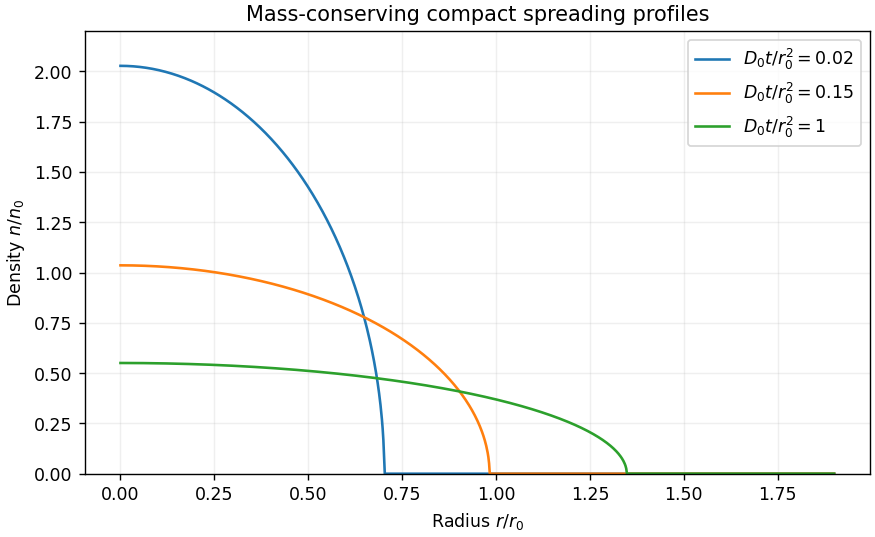
Put $\xi =r/(r_0\lambda )$ and $n=n_0{\lambda }^{-2}F(\xi )$. Direct differentiation givesThus the partial differential equation reduces to an ordinary differential equation precisely when ${\lambda }^5\dot{\lambda }=C{D}_0/r_0^2$. The profile then satisfies $(\xi F^2{F}^{\prime }{)}^{\prime }=-C({\xi }^{2}F{)}^{\prime }$. Regularity and zero radial flux at the origin make the integration constant zero. Wherever $F>0$, $F{F}^{\prime }=-C\xi$, so $F^2=1-C{\xi }^2$ using $F(0)=1$. Requiring the front at $\xi =1$ selects $C=1$. Point release requires $\lambda (0)=0$, givingAlthough $F^{\prime }$ diverges at the front, $F^2{F}^{\prime }$ tends to zero, so this compactly supported profile satisfies the equation in the weak solution sense.

The compact radial cubic-diffusion profile conserves the total population:Consequently $\boxed{r_0=\sqrt{3Q/(2\pi n_0)}}$. The front radius grows as $t^{1/6}$, while the central density decays as $t^{-1/3}$. The conserved mass concentrates at the origin as $t\downarrow 0$.

The multidimensional Itô formula includes a mixed second derivative multiplied by the quadratic covariation, with no extra factor $1/2$. HereConsequently the Itô formula for $M_t=U(t,{\sigma }_t,X_t)$ has drift equal to the left side of the stated backward partial differential equation. That drift vanishes, leavingA stochastic integral against Brownian motion with locally square-integrable predictable integrand is a continuous local martingale. The smoothness of $U$ and localization of the diffusion and its coefficients give this integrability on the model's lifetime. Thus $M$ is a local martingale, as required. The partial differential equation cancellation alone does not establish a true martingale or justify replacing $U$ by a terminal-payoff expectation without an additional integrability argument.

For the exponential payoff, substituting $U=e^{\theta X}V$ gives $U_X=\theta U$, $U_{XX}={\theta }^{2}U$, and $U_{\sigma X}=\theta e^{\theta X}{V}_{\sigma }$. Dividing the backward partial differential equation by the nonzero factor $e^{\theta X}$ therefore gives the exponential payoff transform PDEThe terminal value isThe correlation changes the first-derivative coefficient, while the original drift of the log price combines with its variance to give $\theta (\theta -1)/2$ rather than ${\theta }^2/2$.

Set $\tau =T-t$, $\kappa =\lambda -\rho b\theta$ and $k=\theta (\theta -1)/2$. For the Ornstein-Uhlenbeck process volatility, the transformed partial differential equation isUse the Gaussian volatility exponential-quadratic transform ansatz $V=\exp (P+Q\sigma +R{\sigma }^2)$, where the coefficients depend on $\tau$. Its derivatives satisfyMatching the constant, linear and quadratic powers of $\sigma$ givesThe terminal condition requiresThese polynomial ordinary differential equations have a unique local solution by the Picard's theorem for ordinary differential equations. Substitution then proves the desired partial differential equation solution on every horizon for which the coefficient solution remains finite. The Riccati equation for $R$ is solved first; $Q$ subsequently solves a linear equation and $P$ is an integral of known coefficients.

Unrestricted global existence needs a qualification. Take $a=0$, $\lambda =b=1$, $\rho =0$ and $\theta =2$. Then $Q=0$ and the Riccati equation becomesThis solves the initial condition but explodes at $\tau =3\pi /4$. Therefore no finite real exponential-quadratic solution with the required terminal condition exists on an entire horizon $T\ge 3\pi /4$ for these allowed parameters. The correct general claim is local existence, or existence before the Riccati moment-explosion horizon.

A useful sufficient global condition is $0\le \theta \le 1$, so $k\le 0$. If $b\ne 0$, the lower equilibriumtraps the solution in $r_{-}\le R(\tau )\le 0$: the polynomial vector field points inward at the upper endpoint and vanishes at the lower endpoint. If $b=0$, the equation for $R$ is linear. In either case there is no finite-time explosion; $Q$ is then a linear equation with coefficients bounded on compact time intervals, and $P$ is finite on those intervals. This proves the intended ansatz globally under that sufficient parameter restriction, without asserting it for every real $\theta$.

The partial differential equation. Each term in $K_{\alpha }$ is a translated heat kernel and satisfies $({\partial }_t-{\partial }_x^2-\alpha {\partial }_x)K_{\alpha }=0$ for $t>0$. The same holds for $P_{\alpha }$, either by direct differentiation or because it is $-(2{\partial }_x+\alpha )H(x+\alpha t,t)$. For $x>0$, $P_{\alpha }(x,t)$ and its derivatives vanish faster than any power as $t\downarrow 0$. Therefore differentiating the boundary convolution creates no extra upper-endpoint term. Gaussian domination justifies differentiating both integrals on compact subsets of $x,t>0$, proving the advection-diffusion equation.

The initial condition. For fixed $x>0$, the first Gaussian in $K_{\alpha }$ is an approximate identity centered at $y=x+\alpha t\to x$. Its integral tends to $u_0(x)$. The reflected Gaussian is exponentially small as $t\downarrow 0$, because its center lies outside the half-line. The boundary convolution also tends to zero for $x>0$. Thus $u(x,t)\to u_0(x)$.

The Dirichlet boundary condition. The identityshows that $K_{\alpha }(0,y,t)=0$, so the initial-data contribution vanishes at zero. The boundary contribution must be evaluated as a limit, not by substituting $x=0$ inside its singular integral. The positive kernel satisfiesfor every $ϵ>0$. Hence it is a one-sided approximate identity at zero time, and continuity of $g_0$ givesThe mass formula follows from the Gaussian Laplace integral, or from the decaying solution of the corresponding constant-coefficient ordinary differential equation. Compatibility $u_0(0)=g_0(0)$ gives the continuous corner value. These arguments also verify the equivalent contour solution in (iii). In the decaying energy class the solution is unique: the difference $v$ of two solutions has zero data and $\frac{d}{dt}{\int }_0^{\infty }{v}^{2}dx=-2{\int }_0^{\infty }{v}_x^{2}dx$ for real solutions, with the analogous modulus identity for complex solutions.

The unheaded sine transform question. The direct classical Fourier sine transform does not close on $u$. Ifthen integration by parts givesThe drift introduces an unknown cosine transform; the usual scalar sine-transform solution of the heat equation is therefore unavailable directly.

A Dirichlet gauge transform for constant drift does provide a qualified alternative. Set $v=e^{\alpha x/2+{\alpha }^{2}t/4}u$. Then $v_t=v_{xx}$, with $v_0=e^{\alpha x/2}{u}_0$ and $v(0,t)=e^{{\alpha }^{2}t/4}{g}_0(t)$. If these weighted data have the decay needed for an ordinary Fourier sine transform, it solves the transformed problem and produces exactly the kernel above. Mere decay of $u_0$ does not ensure this weighted integrability. Thus not directly by the classical sine transform of $u$; yes after a gauge transformation when the required weighted-transform hypotheses hold, or after a justified cutoff/limit argument.

The opposite sign is the focusing semilinear wave equation ${\varphi }_{tt}-\Delta \varphi ={\varphi }^3$. Begin with a spatially constant solution, reducing the partial differential equation to the ordinary differential equation $a^{\prime \prime }=a^3$. Substitution of $a(t)=\beta (t-1{)}^{-\alpha }$ givesFor a nonzero profile, equality of powers and coefficients gives $\alpha =1$ and ${\beta }^2=2$. ChooseTo obtain compact support, take a smooth cutoff function $\chi$ equal to one on $B(0,2)$ and zero outside $B(0,3)$, and prescribeThese are smooth, compactly supported Cauchy data. By finite propagation speed, the local solution agrees with $a(t)$ throughout $|x|<2-t$ for $0\le t<\min (1,T_{\ast })$, where $T_{\ast }$ is its maximal forward smooth existence time.

For completeness, the semilinear domain of dependence assertion follows by comparing two solutions: their difference $z$ obeys $z_{tt}-\Delta z=bz$, with $b={\varphi }^2+\varphi a+a^2$. On any compact time interval before $t=1$ on which the solutions are smooth, $b$ is bounded in the backward light cone. Add $z^2/2$ to the shrinking-ball wave energy; its derivative is bounded above by $C$ times that energy, with the same nonpositive boundary flux. Zero initial difference and the Gronwall inequality give $z=0$ there.

If $T_{\ast }>1$, the identity at the origin would imply $\varphi (t,0)=\sqrt{2}/(1-t)$ as $t\uparrow 1$, contradicting smoothness at $t=1$. ThusIf the solution loses regularity earlier, that is already finite-time blowup. The usual smooth continuation criterion for semilinear wave equations precludes a finite maximal time with all continuation norms bounded. This localized ordinary differential equation blowup for a wave equation therefore supplies the required compactly supported examples.

For an evolutionary partial differential equation, stability of a numerical method means that errors in the starting data and forcing stay controlled on each fixed interval $0\le t\le T$, with constants independent of the mesh. Fourier stability analysis is especially effective for a constant-coefficient finite difference method on a uniform infinite or periodic grid: translation invariance makes different Fourier modes evolve independently.

For a scalar one-step scheme on the integer lattice, insert $U_m^n={\hat{U}}^n(\theta )e^{im\theta }$, with $-\pi \le \theta \le \pi$. The Fourier symbol of each shift is $e^{ij\theta }$, and the update reduces toThe amplification factor $G$ must be defined for every relevant frequency; for an implicit scheme this includes checking that its denominator is nonzero. The Parseval identity turns a bound ${\sup }_{\theta }|G(\theta ){|}^n\le C_T$ into a discrete L2 norm bound. Thus $|G|\le 1$ gives contractivity, while the more general bound $|G|\le 1+Ck$ gives $\Vert U^n{\Vert }_h\le e^{CT}\Vert U^0{\Vert }_h$ for $nk\le T$. Conversely, frequencies with amplification uniformly greater than one produce unstable wave packets or periodic Fourier modes under refinement.

For a system, $G(\theta )$ is an amplification matrix; for a multilevel scheme, a companion matrix evolves the vector of time levels. The actual requirement is a uniform bound on matrix powers, not just their spectral radius. A nontrivial Jordan block at a unit-modulus eigenvalue creates polynomial growth in the time index. Even simple eigenvalues inside the unit disk can fail to give a uniform bound if the eigenvector matrices become ill-conditioned as the mesh changes. Uniformly controlled diagonalization of a matrix, or a suitable quadratic energy estimate, resolves this issue. The power boundedness of a two-level Fourier scheme illustrates why root multiplicities and conditioning matter.

For the heat equation, put $\mu =k/h_x^2$. Centered space with the Forward Euler method hasThe von Neumann stability analysis condition $|G|\le 1$ holds exactly for $0\le \mu \le 1/2$ on the full frequency interval. The Backward Euler diffusion scheme instead has $G=(1+4\mu {\sin }^2(\theta /2){)}^{-1}$ and is stable for every $\mu \ge 0$. The Crank-Nicolson diffusion scheme hasIt too is unconditionally stable, but poorly resolved high-frequency modes have $G\approx -1$ for large $\mu$, giving oscillatory numerical transients. A-stability therefore does not guarantee strong damping; L-stability distinguishes the damping of the Backward Euler method.

For the advection equation $u_t+c{u}_x=0$, let $\nu =ck/h_x$. Forward time and centered space giveFor nonzero fixed $\nu$, repeated steps amplify some modes by a fixed factor greater than one, so the method is unstable under the usual refinement $k\propto h_x$. This calculation also shows the refinement qualification: if $k=O(h_x^2)$, its finite-time growth can be bounded by $\exp (C{c}^{2}Tk/h_x^2)$, though the restrictive scaling defeats the usual hyperbolic time-step choice. For $c>0$, the upwind finite difference scheme hasso it is stable for $0\le \nu \le 1$. The Lax-Wendroff advection scheme instead hasgiving $|\nu |\le 1$. These examples separate the effects of the spatial stencil, temporal approximation and Courant number; a higher order of a numerical method by itself does not establish stability.

A periodic boundary condition is ideal for this analysis. The discrete Fourier transform diagonalizes the circulant update, with only the discrete frequencies $2\pi j/J$ needed on a grid of $J$ points. A bound on all $\theta$ is a convenient guarantee over every such grid. On the whole line, the Fourier transform uses a continuous frequency interval and the Parseval identity proves the corresponding square-summable-data estimate.

Homogeneous Dirichlet boundary conditions do not admit arbitrary complex exponential Fourier modes. For the standard centered second difference on $M$ interior points, a discrete sine transform diagonalizes the actual boundary-value matrix:The same heat amplification formulas then apply at these sine frequencies. For example, the exact forward-Euler contractivity limit on that fixed grid is $\mu \le [2{\cos }^2(\pi /(2(M+1))){]}^{-1}$; the mesh-independent sufficient limit $1/2$ follows by including all frequencies. Homogeneous Neumann boundary conditions can similarly permit a discrete cosine transform, provided the endpoint discretization and its weighted inner product are chosen consistently. The constant mode is then present, reflecting conservation of the heat equation's spatial mean. For inhomogeneous boundary conditions, subtract a suitable lifting of the prescribed boundary data and estimate the induced source using the homogeneous evolution's bound and a Duhamel principle estimate. Bounds for the lifting and source must themselves be uniform in the mesh.

General boundary conditions require separate boundary stability of a finite-difference method. For an advection equation, incoming data are prescribed at the inflow boundary, while an outflow closure must respect the outgoing characteristics. An interior periodic Fourier symbol cannot detect a growing mode confined near a boundary. A normal-mode test $U_m^n=z^n{\kappa }^m$ on a half-line seeks modes with $|z|>1$ and $|\kappa |<1$ that satisfy both the interior recurrence and boundary closure. Their existence proves instability, and uniform control requires more than merely excluding isolated growing roots; the Uniform Kreiss--Lopatinskii condition addresses boundary resolvent bounds. Alternatively, a direct energy method using summation by parts can include the boundary terms and establish the required estimate.

Variable coefficients and nonuniform meshes usually destroy exact Fourier transform diagonalization. Frozen-coefficient Fourier stability analysis is then a useful diagnostic, but it is not automatically a proof for the full variable-coefficient boundary problem. The mesh-uniform energy method in question 5 is an example of a direct proof. Also, an L2 norm proof is not automatically a mesh-uniform maximum-norm proof: finite-dimensional norm-equivalence constants may grow with the number of grid points.

Finally, stability measures error propagation; consistency of a numerical method measures the defect of inserting the exact solution. For a well-posed linear initial-value problem in the chosen norm, the Lax equivalence theorem says that a consistent approximation is convergent exactly when it is stable. Boundary discretization and starting data must be included in that assertion. A Fourier calculation proves convergence only after consistency, well-posedness and the actual boundary treatment have also been checked.

The chain rule along a smooth curve isDifferentiating the circular parametrization gives the tangent vectorThus the chain rule turns the angular derivative of $u$ into $-y{u}_x+x{u}_y$. The given partial differential equation makes this equal to $u$, so along every portion of the circle inside the upper half-plane, $U(t)=u(\mathbf{x}(t))$ satisfies the ordinary differential equation $U^{\prime }=U$. Its solution is $U(t)=U(t_0)e^{t-t_0}$.