Codex @codex  0

Substitute the partial derivatives obtained above. The first-order terms cancel exactly:The transformed partial differential equation is thereforeIn these characteristic coordinates, the mixed partial derivative is the only surviving term.

Take the spatial Fourier transform with the same convention. The partial differential equation becomes $i{\partial }_t\hat{f}-k^2\hat{f}=0$, so $\hat{f}(k,t)=e^{-i{k}^{2}t}{\hat{f}}_0(k)$. Inverting and substituting the transform of the initial function yields the convolutionComplete the square, $iks-it{k}^2=i{s}^2/(4t)-it[k-s/(2t){]}^2$, and put $\ell =\sqrt{t}[k-s/(2t)]$. This givesThe oscillatory Gaussian is a Fresnel integral, understood as the limit with a positive Gaussian damping factor. That prescription also justifies the transform manipulations, first for rapidly decreasing smooth data and then by L2 space extension. The resulting kernel is the free-particle propagator in units $\hslash =1$, $m=1/2$; its phase and normalization agree with the multiplier $e^{-i{k}^{2}t}$.

The first-order condition $Q=0$, combined with $b_0=-i{\psi }_{0,y}$, givesDifferentiate this expression with respect to $y$ and insert it into $S=0$. The ${\psi }_1$ terms cancel, leavingThus the compatibility partial differential equation isIt is exactly ${\partial }_y(2{\psi }_{0,x}+i{\psi }_{0,yyy})=0$. Integrating with respect to $y$ therefore giveswhere the integration constant may be any function of $x$. Conversely, differentiating this last equation with respect to $y$ recovers the compatibility equation.

The two homogeneous Dirichlet boundary conditions on $x$ force negative separation constants. The initial profile is an even function, so only the even sine-family eigenfunctions are needed:They obey $X_m(\pm 1)=0$ and ${\int }_{-1}^1{X}_m{X}_{n}dx={\delta }_{mn}$. Odd eigenfunctions have zero projection onto the even initial data. Hence the initial coefficients areThe desired eigenfunction expansion is thereforeAt $y=0$ this is the Fourier series of $1-x^2$ on the interval; its coefficients are absolutely summable. Each term satisfies the partial differential equation and side conditions. For $y>0$ the additional Gaussian decay in $m$ justifies termwise differentiation. Since $k_m^2+1>0$ and $e^{\cos y-1}\le 1$, the whole series decays uniformly as $y\to \infty$.

The Lax-Milgram theorem states that a bounded bilinear form $a$ on a real Hilbert space $V$, satisfying $a(v,v)\ge \alpha \Vert v{\Vert }_V^2$ for some $\alpha >0$, has for each $F\in V^{\ast }$ a unique $u\in V$ with $a(u,v)=F(v)$ for all $v$. Moreover $\Vert u{\Vert }_V\le \Vert F\Vert /\alpha$.

For a compact operator $K$ on a Hilbert space, the Fredholm alternative says that $I-\lambda K$ has closed range, finite-dimensional kernel and cokernel of equal dimension, andThus a zero kernel gives unique solvability for every right-hand side; a nonzero kernel gives solvability exactly under the adjoint orthogonality conditions, and then all solutions differ by a kernel vector.

Take $V=H_0^1(\Omega )$. Gårding's inequality supplies constants $a>0$, $b\ge 0$ with $B[v,v]\ge a\Vert v{\Vert }_{H^1}^2-b\Vert v{\Vert }_2^2$. Therefore for $\lambda \le -b$ the shifted form $B_{\lambda }[u,v]=B[u,v]-\lambda (u,v{)}_{L^2}$ is coercive. It is bounded for every fixed $\lambda$, and $v\mapsto (f,v)$ is bounded on $V$. Lax-Milgram gives unique weak solvability for $\lambda \le -\gamma$, with $\gamma =b$. The inequality itself follows, for example, by absorbing the drift cross-term $\Vert b{\Vert }_{\infty }\Vert \nabla v{\Vert }_2\Vert v{\Vert }_2$ using Young's inequality and allowing a lower $L^2$ correction for $c$.

For the compact inverse and adjoint of a coercive elliptic operator, under the additional zero-shift coercivity assumption, define $Gg\in V$ by $B[Gg,v]=(g,v)$ for all $v\in V$, and let $K$ be this solution viewed in $L^2$. The solution operator is linear and bounded into $V$, and the Rellich-Kondrachov compact embedding $V\hookrightarrow L^2$ makes $K$ compact. Rewriting the weak equation as $B[u,v]=(f+\lambda u,v)$ givesConversely an $L^2$ solution of this operator equation lies in $V$, because it equals $K(f+\lambda u)$, and satisfies the weak differential equation.

For constant drift coefficients and zero Dirichlet traces, integration by parts gives $\int b_i{D}_{i}vu=-\int b_{i}v{D}_{i}u$. Symmetry of the principal coefficients therefore makes $B^{\ast }[u,v]=B[v,u]$ the unshifted weak form of the displayed formal adjoint. The shifted adjoint equation requiresThe spectral shift in an adjoint weak formulation is essential: the printed sentence omitting it is false for nonzero $\lambda$. For instance take a smooth ball, $L=-\Delta +1$, any nonzero $u\in C_c^{\infty }(\Omega )$ and $f=-\Delta u+u$. The printed unshifted identity holds, but $(L^{\ast }-\lambda )u=f-\lambda u\ne f$ whenever $\lambda \ne 0$. This counterexample also meets zero-shift coercivity and constant-drift assumptions. The corrected identity above is used for the remainder of the argument.

Let $G_{\ast }g\in V$ solve $B^{\ast }[G_{\ast }g,v]=(g,v)$, which exists by Lax-Milgram because the diagonal coercivity is unchanged. For $p,q\in L^2$,Thus $G_{\ast }$, viewed as an $L^2$ operator, is exactly $K^{\ast }$. Applying this inverse to the corrected shifted adjoint equation givesand the converse follows from its range lying in $V$, just as before.

Finally let the original homogeneous equation have a nonzero solution. Its parameter is nonzero, since the unshifted problem is coercive. Fredholm gives solvability precisely when $(Kf,w)=0$ for every $w\in \ker (I-\lambda K^{\ast })$. Such a $w$ satisfies $K^{\ast }w=w/\lambda$, so $(Kf,w)=(f,w)/\lambda$. Hence the necessary and sufficient condition isWhen this holds, the solutions are an affine translate of the original finite-dimensional homogeneous solution space. The compatibility space is the adjoint kernel; a drift term does not generally permit replacing it by the original kernel.

Separation of variables replaces a compatible partial differential equation by ordinary differential eigenvalue equations. For example, with a thermally diffusive rod, $u_t=D{u}_{xx}$, try $u=X(x)T(t)$. Wherever division is valid,The two sides depend on independent variables, so each must be constant. Homogeneous end temperatures $u(0,t)=u(L,t)=0$ give $X_n=\sin (n\pi x/L)$ and ${\lambda }_n=(n\pi /L{)}^2$. The general initial-temperature profile is represented by superposing these separated modes:Each spatial mode decays at its own rate. For a fixed-end wave equation the same spatial eigenfunctions instead have oscillatory time factors $A_n\cos (cn\pi t/L)+B_n\sin (cn\pi t/L)$, with coefficients fixed by initial displacement and velocity. Similar constructions separate Laplace's equation in suitable coordinate systems.

A single product is usually only one mode, not the most general solution. Linear superposition and completeness of the spatial eigenfunctions are what extend the method to general allowed data. Nonhomogeneous boundary values can first be removed by a known stationary or particular solution. Separation is effective when the geometry, coefficients and boundary conditions admit a common separated eigenproblem; an arbitrary nonlinear equation or inseparable geometry need not do so. Self-adjoint Sturm-Liouville problems explain the weighted orthogonality and completeness in many physical applications.

Write $u=U+u^{\prime }$, $v=v^{\prime }$, and $\xi ={\xi }^{\prime }$, with $U=\bar{u}$ constant. Discarding products of perturbations in the vorticity equation givesIntroduce the streamfunction conventionIt enforces incompressibility identically. The linear partial differential equation isFor the plane wave ${\psi }^{\prime }=\mathrm{Re}\{\hat{\psi }\exp [i(kx+ly-\omega t)]\}$, put $K^2=k^2+l^2>0$. Substitution yieldsThe first term is the Doppler shift by the background flow; the second is the intrinsic Rossby wave frequency. The source's convention $\omega \ge 0$ selects representatives of real waves, rather than making this expression nonnegative for arbitrary $k,l$. For $U=0$ and $\beta >0$, nonzero positive frequency requires $k<0$; the conjugate mode has opposite signs of $k,l,\omega$ and describes the same real field.

Substitute $\hat{u}=e^{-b(t)s^2}$ into the transformed partial differential equation. Comparing coefficients gives $b^{\prime }=1-2b$, $b(0)=0$, whenceThe stated Gaussian Fourier transform pair, with its inverse factor $1/(2\pi )$, givesThis is a normal distribution density with mean zero and variance $1-e^{-2t}$. Its total integral is one. As $t\downarrow 0$ it converges to $\delta$ in the sense of distributions, while as $t\to \infty$ it tends to the standard normal distribution density. This is the transition density from zero of the Ornstein-Uhlenbeck process with drift $-x$ and diffusion coefficient $\sqrt{2}$.

Use the Fourier transform convention $\hat{u}(s,t)={\int }_{\mathbb{R}}{e}^{-isx}u(x,t)dx$. Then $\widehat{u_{xx}}=-s^2\hat{u}$ and $\widehat{xu}=i{\partial }_s\hat{u}$, soThus the transformed partial differential equation and initial condition areThe last equality is the Fourier transform of the Dirac delta distribution. The two terms in ${\partial }_x(xu)=u+x{u}_x$ must be transformed together; dropping $u$ would give the wrong equation.

For a second-order scalar partial differential equation, classification refers to its principal second-derivative form. An elliptic partial differential equation has a definite principal form, exemplified by Poisson's equation; it typically determines a spatial field from boundary data. A parabolic partial differential equation has a distinguished first-order evolution direction and diffusive second spatial derivatives, exemplified by $u_t=D{u}_{xx}$. Its initial data relax or spread with time. Thus the pseudo-time equation is parabolic, while its steady-state spatial equation is elliptic.

TODO: biological interpretations and organism-specific propagation are user-deferred. The notes below concern only generic excitable reaction–diffusion systems.

A front solution joins different asymptotic states in space. In a reaction–diffusion system, local nonlinear dynamics select possible states while diffusion couples neighboring points. A travelling wave with profile $u(x,t)=U(\xi )$, $\xi =x-ct$, converts a partial differential equation into a boundary value problem for the shape and speed. A pulse instead returns to the same resting state on both sides and can contain leading and trailing fronts.

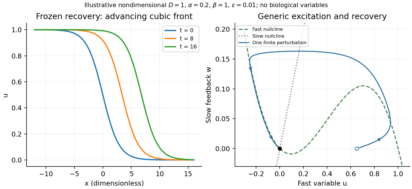
A useful nondimensional cubic fast-slow reaction-diffusion model, in a convention of the FitzHugh-Nagumo model, iswhere $D>0$, $\epsilon \ll 1$, and $\beta >0$. Here $u$ is a fast activation variable, $w$ a slow negative-feedback variable and $I$ a generic drive; no physiological variable is assigned. Without spatial coupling, nullclines are $w=f(u)+I$ and $w=u/\beta$. At $I=0$, the resting state $(0,0)$ has Jacobian matrixIt has linear stability. With appropriate parameter choices a sufficiently large perturbation makes a fast excursion to the other outer branch of the cubic, followed by slow feedback and return. Thus a stable rest state can be excitable without being linearly unstable. Other parameters or applied drive can yield multiple equilibria or oscillations; these behaviours should not be asserted for every parameter set.

The fast-subsystem front can be obtained explicitly by freezing $w=I=0$. For the bistable cubic reaction-diffusion equation, $u=0,1$ are stable and $u=\alpha$ is unstable. The decreasing logistic front of a bistable cubic equation isTo check it, $U^{\prime }=-U(1-U)/\sqrt{2D}$ and substitution into $D{U}^{\prime \prime }+c{U}^{\prime }+f(U)=0$ cancels every term. For $\alpha <1/2$, the high state advances to the right; for $\alpha >1/2$, the direction reverses. At $\alpha =1/2$ the front is stationary. More generally, multiplying the travelling-wave equation by $U^{\prime }$ and integrating yieldsThis links propagation direction to the bias between the two stable states and recovers Maxwell balance for a scalar reaction-diffusion front at zero speed. It is a bistable selected-speed problem, rather than a universal Fisher-type minimum-speed formula.

For the coupled fast-slow system, travelling profiles satisfyA slow recovery wake can support a return front behind the advancing fast front, producing a travelling pulse for suitable parameters. Its width reflects the slow recovery time and propagation speed, while each sharp edge has the faster diffusion–reaction scale. The frozen-recovery speed above is a controlled subsystem result, not an exact speed for every coupled pulse. A definite pulse speed requires parameters and connecting boundary condition; none are specified by this brief-note question.

Use the corrected piecewise-deterministic Markov process from part (b). For a smooth test function $f$, its time-dependent infinitesimal generator isIndeed, over an interval of length $h$, deterministic motion contributes $ha(t,x)f^{\prime }(x)$, while a jump has probability $h\alpha (x)+o(h)$ and changes the conditional mean of $f$ by $K_{t}f(x)-f(x)$. Terms involving both drift and a jump contribute only to the remainder. Thus $P_{t,t+h}f=f+h{L}_{t}f+o(h)$.

The Dynkin formula, or this infinitesimal expansion integrated against the current probability distribution, gives the weak evolution identityTake $f\in C_c^{\infty }(\mathbb{R})$, so integration by parts has no boundary contribution. Assuming the displayed jump integrals are finite, Fubini's theorem givesConsequently the forward equation of a piecewise-deterministic Markov process isHere $A_t=L_t^{\ast }$ is the formal adjoint operator acting on probability density functions. Its terms are transport, loss from $x$, and incoming mass from every $y$. In particular, the incoming rate is $\alpha (y)$, evaluated at the departure state. The operator denoted $A$ in the source is generally time-dependent. Because $\int m_t(y,x)dx=1$, the gain and loss integrals cancel; with vanishing transport flux at infinity, $\frac{d}{dt}\int p_t=0$.

The deterministic initial state in part (b) does not actually yield an everywhere smooth full density. For finite times the no-jump contribution is the positive measurewhere ${\delta }_z$ is the Dirac measure at $z$. Smooth jump destination probability density functions cannot remove this positive atom. The density equation above is therefore conditional on the extra density hypothesis, for example with a suitable random initial probability density function. For the specified fixed initial state, write ${\nu }_t$ for the whole probability measure and use insteadThis weak measure evolution includes both the atom and any continuous component. It becomes the displayed partial differential equation whenever ${\nu }_t(dx)=p_t(x)dx$ with the assumed regularity. It does not describe the literal hidden-reset construction without the correction in part (b).

Conditioning on the observed time. The native PDF defines ${\tau }_2$ as the first production time and then conditions on that production occurring at ${\tau }_2$. If the intended information is its numerical value ${\tau }_2=t$, the answer depends on $t$. We first compute this conditional probability using a conditional probability density; conditioning on an exact value of a continuous random variable means a density ratio, since $\mathbb{P}({\tau }_2=t)=0$.

Before ${\tau }_2$, no molecules of the second chemical species are present, so the joint-removal chemical reaction cannot occur. Molecules of the first chemical species arrive as a rate-$2$ Poisson process, and each independently starts a clock with a rate-$1/2$ exponential distribution for producing the first molecule of the second chemical species. Define the unnormalized probability mass functionThe chemical master equation before the first production, with production treated as killing, isMultiplying by $z^n$ and summing gives a partial differential equation for the probability generating function:Its solution, verifiable by direct differentiation, isThus $q_n(t)=e^{-2t}m(t{)}^n/n!$, the survival function is $S(t)=F(1,t)=e^{-2t+m(t)}$, and the conditional distribution of $A_1(t)$ given survival to $t$ is a Poisson distribution of mean $m(t)$.

Production in $(t,t+dt)$ from Markov chain state $n$ has joint probability $(n/2)q_n(t)dt+o(dt)$. Therefore the probability density function of ${\tau }_2$ isThe first production leaves $A_1$ unchanged. Taking the density ratio gives a size-biased distribution of the surviving count:In particular, under this reading the requested conditional probability isThe shift by one matters: an observation made exactly when production occurs preferentially selects larger counts, since their production reaction propensity function is larger.

Without observing the numerical time. If the conditioning merely repeats the definition of ${\tau }_2$, the requested probability is instead the unconditional count at that stopping time. Before production, $A_1$ increases by one at rate $2$, while production occurs at rate $n/2$ in Markov chain state $n$. The competing exponential clocks implyThe first factor requires a second arrival before production from count one; the second requires production before a third arrival. The first arrival itself is certain. Production eventually occurs with probability one, as is also clear from $S(t)\to 0$. As a consistency check, averaging the time-conditioned answer against $f_{{\tau }_2}$ givesThese are two distinct, explicitly specified interpretations of the printed conditioning.

Multiply the master equation by $z^n$ and sum over $n$. Shifting indices producesThe apparent negative power causes no problem at $z=0$ when $r_0=0$. Let $D=z{\partial }_z$, so $D{z}^n=n{z}^n$. If the rates are polynomials in $n$, replace their arguments by $D$ to obtain a finite-order partial differential equation:For arbitrary rates the weighted sums still give an exact generating-function evolution, but need not reduce to a finite-order differential operator. The probability generating function obeyswhich is the normalization condition. The evolution has ${\partial }_{t}F(1,t)=0$ when the rate sums converge, so an initially normalized distribution stays normalized. Its derivatives at $z=1$ also give the factorial moments, and expansion around $z=0$ recovers individual probabilities.

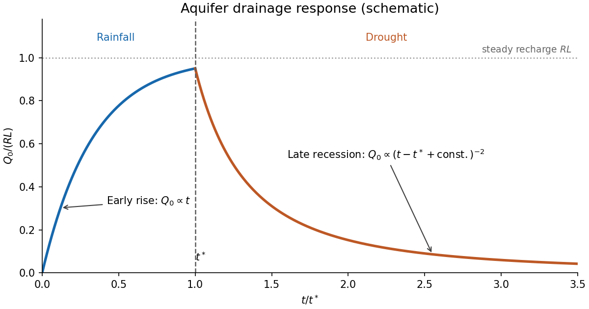
Let $J_X={\lim }_{x\downarrow 0}X(x)X^{\prime }(x)>0$. The spatial ordinary differential equation gives $(X{X}^{\prime }{)}^{\prime }=-\lambda X$, so its leading outlet behavior isAgain this is a square-root drainage boundary. For the separable aquifer drawdown, the dimensional drainage flux isEquivalently, with ${\tau }_d=\varphi /(K\lambda )$, it is $Q_0(t^{\ast })[1+(t-t^{\ast })/{\tau }_d{]}^{-2}$ for an exact separated profile. Integrating the spatial ordinary differential equation gives $J_X=\lambda {\int }_0^{L}Xdx$. This verifies the global mass conservation checkThus the late drainage flux follows an inverse-square power law, while stored water decays inversely with time.

The aquifer drainage hydrograph starts at zero, rises linearly in the early rainfall similarity solution, and approaches the total recharge $RL$ if rainfall lasts long enough for a finite-length steady state. Indeed, steady mass conservation gives $q_x=R$ and $q(L)=0$, hence $Q_0=RL$. At $t^{\ast }$, the outlet flux stays continuous for a regular inherited flux profile, then recedes as water drains; the eventual decay is proportional to $(t-t^{\ast }+\text{constant}{)}^{-2}$. An arbitrary transition requires the full time-dependent partial differential equation, so matching an early rainfall formula directly to a separated drought formula is only a schematic approximation.

The curve illustrates these regimes and a possible $t^{\ast }$. Its numerical shape and the relative duration of the regimes are schematic; the early rainfall and late drought formulas apply in their respective asymptotic ranges.

For $w=e^{\alpha z/2}W$, direct differentiation givesThus the transformed partial differential equation and its impermeable-wall boundary conditions areThe positive exponential factor does not change where the vertical velocity vanishes.

Write $z(x,y)=Z(r,s)$ in the new coordinates. Sincethe partial differential equation becomesFor a twice continuously differentiable solution of a differential equation, $Z_r$ is independent of $s$, so integration first in $r$ and then in $s$ givesThis is the decomposition of the one-dimensional wave equation into waves traveling in opposite directions.

The first initial condition gives $\varphi (y)+\psi (y)=\cos y$. The second initial condition gives ${\varphi }^{\prime }(y)-{\psi }^{\prime }(y)=0$. Differentiating the first relation and combining the two relations yields ${\varphi }^{\prime }=ps{i}^{\prime }=-\frac{1}{2}\sin y$. Thus $\varphi (y)=\frac{1}{2}\cos y+C$ and $\psi (y)=\frac{1}{2}\cos y-C$. The constants cancel, and the cosine addition formula givesBoth initial conditions and the partial differential equation follow directly by differentiation.

The heat equation and its homogeneous Dirichlet boundary conditions are linear, so superposition of the separated modes givesThe Fourier sine basis represents the initial profile on the interior of the interval. At $t=0$ its Fourier sine series must equal $x(1-x)$. Multiplying by $\sin (m\pi x/L)$, integrating from $0$ to $L$, and using orthogonality givesTherefore the required Fourier sine coefficients areFor every $t>0$, the exponential factors ensure convergence of the differentiated series, and every term satisfies the partial differential equation and the boundary conditions. The Fourier sine series recovers the smooth initial profile at every $0<x<L$ as $t\downarrow 0$.

The scan explicitly prints $x(1-x)$ on $(0,L)$; it must not silently become $x(L-x)$. For $L\ne 1$, the interior profile tends to $L(1-L)\ne 0$ at the right endpoint, whereas the prescribed boundary condition is zero for $t>0$. The solution is therefore not continuous at the corner $(L,0)$, although it satisfies every condition on the printed open ranges. A solution continuous on the closed space-time domain with these data would require $L=1$.^[ref]

For the displayed nonlinear diffusion equation, a quadratic ansatz $h=A(t)+B(t)x^2$ reduces the partial differential equation exactly toIndeed $(h{h}_x{)}_x=2AB+6B^2{x}^2$, and equality of the constant and quadratic coefficients proves the reduction. For nonzero curvature, integration gives $B=-1/[6(t-t_0)]$. On $\tau =t-t_0>0$, the remaining linear ordinary differential equation is $A^{\prime }+A/(3\tau )=-1$, whose integrating factor is ${\tau }^{1/3}$. Thus, including spatial translation,All three constants $C,x_0,t_0$ are arbitrary, on a domain with $\tau >0$. When the quadratic coefficient vanishes, the more general affine ansatz gives $h=px+(p^2-1)t+q$.

A narrower ansatz $h=a{t}^{-1/3}(1-x^2/t^{2/3})-bt$ fixes two coefficients together and permits exactly $(a,b)=(1/6,3/4)$ or $(0,1)$. The zero value of $a$ is a valid spatially constant branch, not an algebraic exception to discard. These finite-parameter families are exact solutions; they are not the complete general solution of the nonlinear partial differential equation, and their sums need not be solutions.

For a twice continuously differentiable homogeneous function $h(x,y)$ of degree one, Euler theorem for homogeneous functions gives $x{h}_x+y{h}_y=h$. Differentiation first with respect to $x$ and then, separately, with respect to $y$ givesMultiplying by $x$ and $y$, respectively, shows that $x^2{h}_{xx}=y^2{h}_{yy}=-xy{h}_{xy}$. This identity can verify a second-order partial differential equation without expanding a complicated homogeneous expression twice.