Source bundle pages 123–128. The paper cover establishes 2022; the attachment filename uses 2021. Solutions use the symbols of the source, with corrections and approximation limits identified where needed.
Take along a horizontal gap and perpendicular to its plates, with . Assume a Newtonian fluid, stationary plates, a steady flow, a laminar flow and a fully developed flow away from the entrances and side edges. The no-slip boundary condition holds on both plates. Any transverse gravity is absorbed in the hydrostatic pressure; there is no imposed transverse through-flow. Translational symmetry and the no-penetration boundary condition then give . The Navier-Stokes equation reduces toTwice integrating gives the plane Poiseuille flow:The volumetric flow rate through one gap isThere are internal gaps. Their total cross-sectional area is , because the plate thickness is negligible, so the Darcy velocity isThus the permeability of a porous medium has the dimensions of squared length. If finite plate thickness were included, the Darcy velocity averaged over the whole manifold would also contain its porosity.
Both the local acceleration and the convective acceleration vanish: and . The dominant balance is therefore between the pressure gradient and viscous stress, with no inertia contribution in this fully developed solution. This exact cancellation does not guarantee that arbitrary large-Reynolds number realizations remain laminar flows; entrances, disturbances and turbulence can invalidate the assumptions.
Use a fixed representative volume containing many pores. Let be the porosity and let be the Darcy velocity, defined per unit total area. The conservation of mass isThe solid matrix is rigid and fixed, and the liquid is fully saturating and has constant mass density, so the stored mass on the left is constant. Microscopic internal liquid-solid boundaries contribute no through-flux by the no-penetration boundary condition. Applying the divergence theorem to the external flux givesSince the representative volume is arbitrary, the macroscopic continuity equation isThere is no extra factor of in the flux: that factor is already incorporated in the definition of the Darcy velocity. A compressible liquid or deformable matrix would require retaining the storage term.
Under spherical symmetry, the continuity equation and Darcy's law giveHence , and integrating the pressure gradient from infinity givesThe boundary condition at fixes . Therefore spherical Darcy injection hasHere is the superficial Darcy velocity, not the pore velocity .
For the comparison, assume geometrically similar pore networks, equal porosity, the same source radius and far boundary geometry, and equal pump efficiency. Dimensional analysis then gives with the same dimensionless factor. ConsequentlyAt a fixed desired volumetric flow rate, the required excess pressure and pumping power areAquifer A requires half the pumping power at equal throughput, or half the energy to inject the same volume over the same time. This compares the excess pressure-volume work dissipated by the Darcy flow; any different baseline compression or other plant costs need separate accounting.
The imposed comparison matters. At fixed , A takes twice the volumetric flow rate and twice the instantaneous power, but the same excess energy per injected volume. The pore spacing alone does not determine permeability of a porous medium if network geometry or porosity changes; without the geometric assumptions the preference cannot be inferred from alone.
For the common constant mass density, the background hydrostatic pressure satisfies . Define the excess pressure . In Darcy's law, the background pressure gradient cancels gravity:If the source imposes the same excess pressure relative to the local hydrostatic pressure everywhere on its spherical surface, , the spherical Darcy injection result survives exactly:It is important to specify what is maintained on the source. A literally uniform absolute pressure on a finite sphere centered at instead gives , where is measured from the upward vertical. The decaying harmonic function outside the sphere is thenand thereforeThis supplies a concrete exception to an unqualified claim that gravity leaves the radial flow unchanged. The additional dipolar contribution has zero net volumetric flow rate, so still holds. Equal injected and resident mass densities are essential to the background cancellation.
At a fixed point beside a river, the Eulerian coordinate description measures . Its local acceleration measures change at that fixed point. Following a floating parcel gives a Lagrangian trajectory satisfying . The chain rule gives its physical material acceleration:The extra term is the convective acceleration. For a river that narrows steadily, an observer at one fixed position measures a constant velocity, yet a parcel speeds up as it reaches the narrowing. A parcel following a steady bend also experiences a centripetal acceleration even when its speed is constant. An Eulerian calculation of the physical acceleration must include the same convective acceleration; the two descriptions do not predict different forces.
Choose the stream function convention , , so that this is an incoming stagnation point flow rather than the reversed flow. The velocity field isAt the plate , satisfying the no-penetration boundary condition. The nonzero tangential velocity is permitted for an inviscid flow; the no-slip boundary condition is not imposed on the Euler equations for an inviscid fluid.
The steady convective acceleration is . Thus the Euler equations for an inviscid fluid requireIntegrating givesThe printed formula omits from its quadratic term. The source uses physical pressure, not pressure divided by mass density, as is clear from its term and its Navier-Stokes equation. The omitted factor is also required by dimensional analysis. For a concrete substitution check, the printed expression gives rather than the required when in the chosen numerical units.
A stationary viscous wall imposes the no-slip boundary condition, , whereas the outer inviscid flow has . At large Reynolds number, the transition is confined to a thin viscous boundary layer, where normal velocity gradients amplify the otherwise small viscous term.
Take a horizontal scale , an outer speed , and a boundary layer thickness . The continuity equation gives . Write and . The tangential Navier-Stokes equation has scalesBalancing convective acceleration with normal viscous diffusion gives . The leading tangential equation and incompressible flow constraint areHere and below is the kinematic viscosity, while is the horizontal velocity.
For the normal equation, first remove the hydrostatic pressure by writing . Normal inertia and normal viscous terms are , so the change of across the layer is only . Matching to the outer pressure therefore makes the leading excess pressure independent of :The outer expression similarly has . Thus the printed conditionis a leading-order boundary layer matching statement, with the smaller normal dynamic terms discarded on both sides. It is not an exact identity at the next order. In particular, retaining the outer while dropping normal inertia and normal viscous terms inconsistently mixes orders. The tangential driving term is unambiguous: .
Use the same stream function convention and denote differentiation with respect to the dimensionless variable by a prime. The proposed similarity solution givesIts continuity equation holds identically. Substitution in the tangential Prandtl boundary-layer equation givesChoose the constant scale . The Hiemenz flow equation and its boundary conditions areThe first two conditions impose the no-penetration boundary condition and no-slip boundary condition. The last matches the tangential outer velocity. One also has and . It is too strong to impose : the displacement thickness generally permits a constant offset, .
The normal Navier-Stokes equation makes the approximation in part (c) explicit. With this similarity solution, it givesAt the wall this differs from by . This is a concrete next-order counterexample to interpreting the printed normal pressure gradient equality exactly; the tangential Hiemenz flow equation remains valid at its stated order.
The Hiemenz flow profile changes on , so its boundary layer thickness isA specified edge convention, such as , introduces an order-one numerical multiplier requiring the profile to be solved. Scaling alone does not determine that multiplier. The result has no separate dependence on , , or at fixed kinematic viscosity. At fixed dynamic viscosity, it is .
The viscous diffusion time across a thickness is ; the imposed strain has time scale . Their balance sets the thickness. Increasing kinematic viscosity spreads the layer, while increasing the imposed velocity gradient presses the layer toward the wall. The outward tangential velocity increases as , so the decreasing travel time per unit distance offsets the usual downstream broadening.
For a conventional estimate of transition to turbulence, form the local horizontal Reynolds number:If transition is assumed to occur at an empirical value , thenA rough borrowed threshold of order – would give of order –. This is a heuristic estimate, not a universal stability prediction: the accelerating outer flow and favorable pressure gradient can delay transition, and disturbance amplitudes and wall roughness matter. Simply setting locates failure of the thin-layer approximation near the stagnation point, not onset of turbulence.
Each layer has constant mass density, initially negligible velocity and hence zero vorticity. Its Euler equations for an inviscid fluid have a conservative gravitational body force, so Kelvin's circulation theorem preserves zero bulk vorticity. In a simply connected layer, the irrotational flow therefore has . The incompressible flow condition givesThis applies while the ideal layerwise solution is smooth. It allows an interfacial vortex sheet; it does not assert that the whole two-fluid flow has zero vorticity or that a smooth interface must exist for arbitrarily long times.
The rigid wall no-penetration boundary conditions arewith boundedness and at for regular axisymmetric fields. For a small interface displacement and small slope, linearization of the kinematic boundary condition about givesThe small-slope condition is an additional requirement for high-wavenumber modes: , not just .
Choose the unperturbed hydrostatic pressures as . The linearized Bernoulli equation gives the pressure perturbation , after absorbing spatially constant gauges into . Since surface tension and viscous normal stress vanish, pressure continuity on givesorThe initial velocity is zero, so . Separate conservation of mass in each closed layer also requires relative to the initially horizontal interface.
Write using the Bessel function of the first kind. The wall boundary conditions at selectBecause , the sidewall no-penetration boundary condition requireswhere are the positive zeros of . These radial eigenfunctions automatically preserve layer volume becauseThe constant radial mode cannot change the interface height in a closed tank: the Laplace equation and the impermeable lids then give zero vertical velocity, and a uniform displacement would change each layer's volume.
The kinematic boundary condition fixesThus the interface values are and . Substitution in the normal stress condition gives the finite-depth Rayleigh-Taylor dispersion relation:soHere is the Atwood number. Every allowed mode has a positive growth rate and is subject to Rayleigh-Taylor instability. Since , shorter radial scales grow faster. The limits areThere is no fastest finite wavenumber in the ideal sharp-interface model without surface tension, viscosity or diffusion. The zero-initial-velocity condition uses both exponential branches: an initial mode evolves as . If the mass density ordering were reversed the same calculation would give oscillatory stable modes; equal mass densities give neutral modes.
For an inviscid flow, the force per unit volume is . The gravitational acceleration has zero curl. Using the curl product rule,The supplied two-dimensional vorticity equation therefore becomesThe out-of-plane vorticity has no stretching term in this two-dimensional setting. The source is baroclinic vorticity generation: differently directed mass density and pressure gradients generate rotation even from zero initial vorticity.
For an explicit sign check, set , with upward. A thin smoothed interface has , with . If denotes the total pressure evaluated on the interface, then within the thin layer andIntegrating through that layer and taking its thickness to zero gives the vortex sheet strength and its linear evolution:For a growing Fourier mode, the potentials from the preceding calculation with replaced by giveThus the right-hand descending slope of a light-fluid crest produces positive , while the left-hand ascending slope produces negative . Their induced velocity raises the light-fluid crest and lowers the heavy-fluid trough, increasing the slope and generating more vorticity. This is the positive feedback underlying Rayleigh-Taylor instability.
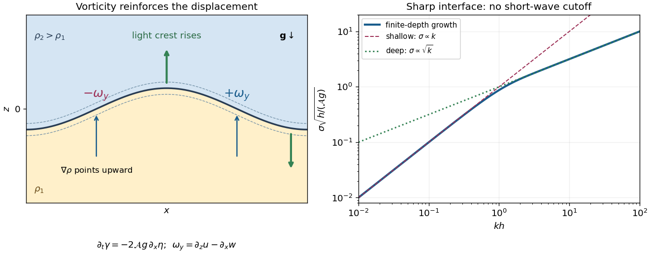

One can close this mechanism quantitatively. For , the kinematic boundary conditions give . Combining with the sheet-generation equation givesFor , the lids confine motion throughout both layers and horizontal redistribution is slow, yielding . For , motion is localized within depth on each side. Less fluid must accelerate at shorter wavelength, giving . Since , the ideal growth rate increases with with no short-wave cutoff.
The sharp-interface result requires for the smoothed layer. When becomes order one, it no longer applies. A smooth adverse mass density gradient has a local overturning time of order rather than the unbounded sharp-interface rate. Finite molecular diffusion also relaxes small-scale mass density perturbations on a time of order , and viscosity, if included, damps small-scale velocity. Weak diffusion motivates the thin-layer picture; it does not justify extrapolating the discontinuous dispersion relation to arbitrary .
A small Reynolds number, , means that inertia is small compared with viscous forces. It can arise from small speed, small length or large dynamic viscosity. Examples are the locomotion of a microswimmer and the slow sedimentation of a small particle in a viscous liquid.
To neglect local acceleration as well, an externally imposed time scale must satisfy . This holds for a steady flow or a sufficiently slowly varying quasi-steady Stokes approximation. Small Reynolds number alone is insufficient for that extra step. For an incompressible flow with constant material coefficients and uniform gravity, the Navier-Stokes equation then reduces to the Stokes equation:Taking the divergence and using commuting spatial derivatives givesTaking the curl, which annihilates the pressure gradient and uniform gravitational force, givesThese are the Harmonic pressure and vorticity in Stokes flow results.
A concrete counterexample to inferring both solely from small Reynolds number is Stokes' second problem: an oscillating plate with arbitrarily small velocity amplitude has negligible inertia, but is nonzero. Its vorticity is not a harmonic function. The quasi-steady qualification is therefore necessary.
For an axisymmetric field without azimuthal motion, the divergence in spherical coordinates isSubstituting the given axisymmetric stream function representation givesThus incompressible flow is automatic.
The velocity components are laboratory-frame components resolved about the instantaneous bubble center. The center itself translates with . The kinematic boundary condition for a spherical interface givesFor negligible internal dynamic viscosity, continuity of tangential traction imposes zero tangential shear stress, rather than a prescribed tangential velocity. In terms of the strain-rate tensor,Equivalently, . Axisymmetry gives , and the far-field boundary condition is . There is no no-slip boundary condition on a clean bubble; the liquid can slip tangentially relative to the translating interface.
These are the conditions of the prescribed-sphere clean-bubble Stokes drag model. A genuinely free bubble also requires a normal stress balance. If one additionally insists on spatially uniform gas pressure, while removing both surface tension and the variation of hydrostatic pressure, that extra condition is incompatible with the translating spherical solution in part (c). The approximation must therefore be understood as computing drag on an imposed spherical interface, or as retaining the normal balancing effects when checking a free bubble.
Differentiating the axisymmetric stream function givesThe normal kinematic boundary condition fixes , soBoth velocity components vanish at infinity, and the axisymmetric stream function is regular at the polar axes. The tangential component of the strain-rate tensor vanishes everywhere:Thus the stress-free boundary condition is satisfied. The vorticity is , and the supplied dipolar pressure is consistent with the Stokes equation.
Use the Newtonian fluid stress tensor . At the bubble surface,The vertical force exerted by the liquid is the integral of the vertical traction:Since the integral is , the drag is downward and has magnitudeThe constant pressure integrates to zero force. The pressure perturbation contributes and the normal viscous stress contributes ; there is no tangential traction contribution.
For the free-interface qualification in part (b), the calculated normal traction at and differs by . It cannot equal a single uniform gas pressure if every restoring effect is discarded. Restoring the external-minus-internal variation of hydrostatic pressure supplies a term . It cancels the dynamic normal traction at the terminal velocity , consistent with a spherical clean bubble without surface tension. This distinguishes the drag calculation from the extra conditions needed for a freely rising bubble.
Retain the clean-bubble approximation used in parts (b) and (c), with constant mass densities and diffusion coefficient. For a spherical bubble,ConsequentlyThe buoyancy minus bubble weight is . Balancing it against the clean-bubble Stokes drag gives the instantaneous terminal velocitySet at the initial position. Combining this with the dissolution equation gives and hence the dissolution-limited bubble rise lawThe expression applies until the bracket vanishes. The rise speed decreases continuously as the bubble shrinks. Equivalently, , providing a direct check on the elimination of time.
The phrase “constant terminal velocity” must here mean rapid adjustment to a force balance at each radius. A literally time-independent speed is incompatible with that balance because . If instead an external mechanism maintained a fixed , the distinct result would be and . In particular, holding the initial terminal speed fixed doubles the predicted rise distance; it is not the freely rising shrinking-bubble model.
Using the supplied values and givesEquality means dissolution exactly on arrival at the surface; dissolution strictly before arrival needs a greater initial depth. This is a formal low-Reynolds number estimate. The same values predict and a radius-based Reynolds number ; the diameter-based value is about . Neither is . Thus the numerical input does not consistently satisfy the Stokes flow assumption initially, and the result should not be presented as an accurate oceanic prediction. Within the stated ideal model, bubble compression, contaminants and changes in dissolved-gas concentration are also excluded.
The cover dates this paper to 11 June 2021 despite the attachment filename. Solutions identify a false printed biharmonic equation identity, retain the stipulated drop curvature approximation explicitly, and state the conditions needed for the final Joukowski map.
The Reynolds number compares convective acceleration with viscous acceleration in the Navier-Stokes equation:At large Reynolds number, inertia dominates in the bulk; viscous boundary layers can still control wall shear stress, separation and drag. Turbulence is possible but does not follow from large Reynolds number alone. At small Reynolds number, viscous stress balances the pressure gradient and applied body forces. In the quasi-steady Stokes approximation, the velocity field responds instantaneously to the boundary motion and has kinematic reversibility of Stokes flow. Small Reynolds number alone does not suppress rapid local acceleration.
For a swimmer, take a characteristic length and speed . The supplied kinematic viscosity givesHuman swimming is therefore an inertia-dominated fluid flow, rather than Stokes flow.
The divergence in polar coordinates and the given streamfunction convention yieldThus the incompressibility condition holds wherever the mixed partial derivatives commute. The vertical vorticity isNeglecting both inertial terms in the Navier-Stokes equation, for constant dynamic viscosity and mass density, gives the Stokes equation:Its curl eliminates the pressure gradient and the uniform gravitational body force, so . Hence the biharmonic streamfunction satisfiesThis conclusion requires the quasi-steady Stokes approximation. If local acceleration were retained, the corresponding planar vorticity equation would instead be .
Write , positive on opening. The no-slip boundary condition equates the fluid velocity with each plate's velocity:The upper condition is a moving-wall no-penetration boundary condition, not zero normal velocity in the laboratory frame. At the hinge the velocity tends to zero. With the arbitrary constant of the streamfunction chosen so that , these conditions becomeA changing angle cannot give a literally steady flow in fixed coordinates. We interpret the stated steadiness as the quasi-steady Stokes approximation at each instantaneous .
The printed expression is not biharmonic. To test it without reproducing the source formula, write its bracket as and its streamfunction as . For any angular function , the Laplacian givesAt the concrete angle , differentiation of the printed bracket givesFor example, at the interior point ,The printed bracket does satisfy and , so its boundary velocities would require . Satisfying these boundary conditions does not cure its nonzero biharmonic operator. The stated series is likewise not a general biharmonic basis: its term already fails the displayed test. The separated polar solutions of the biharmonic equation contain additional radial powers; for the required dependence, the angular basis is .
The corrected slowly opening Stokes wedge similarity solution follows by setting . The biharmonic equation gives . The two lower-wall conditions reduce its general solution toThe upper-wall condition fixes the ratio of and , and fixes their scale. An expression that also remains finite at isFor , its denominator is positive: the derivative of is . Direct differentiation verifies all four boundary conditions and the biharmonic equation. The resulting velocity components are and .
For a fixed angle of order one, , so the local Reynolds number is . One breakdown length is thereforeA second is the geometric length , where is the distance to the radial ends and the spanwise width. At , matching to the surrounding bath or three-dimensional end flow matters. Thus is required for this local two-dimensional Stokes flow, with angle-dependent factors in the inertial estimate. Ideal infinite plates remove the geometric cutoff but not the inertial one.
There is also a temporal restriction: the relevant viscous diffusion time must be short compared with the time over which the shape and its velocity field change appreciably. Using as a conservative diffusion length gives . For order-one angles and constant , gives the same scale as ; narrow angles require using their actual gap and angular factors rather than extrapolating this order-one-angle estimate.
Take outward radial volume flux per unit width as positive. The streamfunction in polar coordinates immediately givesFor spanwise width , the volumetric flow rate is . The wedge inside radius has cross-sectional area , whose rate of increase is . Opening therefore draws in exactly the volume needed to fill the expanding wedge; closing expels it. This is also a direct check of conservation of mass for the moving control volume. It follows from the wall boundary conditions and remains true even though the printed interior streamfunction is erroneous.
Given an admissible velocity field, recover the pressure gradient from the Stokes equation, , and integrate it, fixing the additive constant by matching to the bath pressure near the open ends. The biharmonic equation ensures the compatibility of this integration. For a freely moving hinge, the laboratory velocity field also contains the unknown rigid translation and rotation. Solve the interior and exterior Stokes flows with these wall velocities, then impose zero total external force and torque on the complete apparatus if its motor supplies only internal actuation. The pinned solution alone cannot determine that free motion.
At a fixed angle, the actuation velocity scale is . The Stokes equation gives . Integrating normal traction over a plate of length gives a force per unit width of scalewith a dimensionless signed coefficient depending on geometry and exterior matching. Normal viscous stress has the same dimensional scale and is included in . The force reverses when the actuation reverses. A narrow gap can make large.
More specifically, the corrected local streamfunction gives, up to a reference pressure,Indeed, inserting into the vector Laplacian gives and . For , opening produces reduced pressure toward the hinge when matched at . The logarithmic singularity is integrable: , consistent with the stated force scale. A real hinge regularizes the singularity; the local formula is not a full end-matched solution.
The scallop theorem applies to a single periodically actuated hinge in a stationary Newtonian fluid with negligible fluid and body inertia. At each shape, Linearity of Stokes flow makes its rigid velocity proportional to . Closing retraces the sequence of shapes and reverses the corresponding motion, irrespective of different opening and closing rates. The hinge may move during each half-cycle, butA motor can generate instantaneous forces and consume energy through viscous dissipation without producing sustained swimming. Additional independently controlled shape changes, appreciable inertia, or a fluid with memory would require a different analysis.
Compressing a small region raises its mass density and, for positive compressibility, its pressure. The outward pressure gradient force accelerates neighbouring fluid elements. Their outward motion compresses fluid farther away, carrying the disturbance outward. The original compressed region relaxes; inertia allows the fluid motion to continue beyond zero excess pressure, producing a rarefaction and a restoring pressure gradient force. Elastic compression and inertia therefore support a propagating longitudinal wave.
In a local planar description with acoustic displacement ,so . The speed of sound is a propagation speed, whereas the acoustic particle velocity is the small back-and-forth motion of the medium. In linear acoustics, energy travels with the disturbance without first-order net transport of the fluid over a wave period.
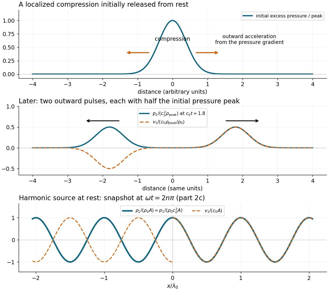

For one-dimensional inviscid flow, conservation of mass and the Euler equation areSubstitute and the stated background-plus-perturbation expressions. Dropping products of perturbations gives the linearizationThe Taylor expansion of the equation of state givesSince the background coefficients are constant, commutes with . Applying to the linearized continuity equation and using the linearized Euler equation therefore yieldsThis is the convected acoustic wave equation: in the coordinate , it becomes the ordinary one-dimensional wave equation. Positive is required for propagating sound waves.
Use a plane wave proportional to . Substitution into the convected acoustic wave equation gives the dispersion relationThe two branches have signed phase velocities and group velocities . On a branch with , , the linearized Euler equation givesIn subsonic flow with , the absence of wave reflection selects the outgoing branch on each side:For , take real and positive by choosing the source phase, and put . At , the requested spatial profiles areFor complex , retain instead. The normalized sound pressure and acoustic density perturbation lie on the same even cosine curve. The acoustic particle velocity follows that curve on the right and its negative on the left, as in the figure in part 2(a). Compressed fluid moves away from the source on both sides. These are two outgoing travelling waves, not a standing wave. The ideal point loudspeaker supplies the discontinuity of velocity at ; the source-free equations apply on either side of it.
Take the wind to blow toward positive , so . In subsonic flow, both stationary observers record the source angular frequency and, for the imposed density boundary data, the same acoustic density perturbation amplitude . Their spatial records distinguish the wavelengths and directions:The downstream pattern moves at and the upstream pattern at signed velocity . Thus the downstream observer sees longer wavelengths while the upstream observer sees shorter ones. The interval containing multiple wavelengths lets each measure the spatial spacing and its direction of travel. The arrival delays at are and respectively; after arrival their temporal traces differ by these propagation phases, not by temporal frequency.
In supersonic flow, both characteristic curves have positive slopes . With an initially undisturbed upstream region, the observer at sees no source-generated disturbance. The observer at can see two downstream travelling waves, withThe faster signal arrives first, at ; the slower one arrives at . Once both are present, their different wavenumbers can produce spatial modulation, while the time dependence at a fixed position remains harmonic with angular frequency .
There is a qualification to the source data: the single prescribed value of fixes only . It does not determine the two complex amplitudes separately. A second source condition, such as its downstream acoustic particle velocity with amplitude , or a specified mass/force source model, is needed. Consequently two downstream branches are allowed; the stated density data alone do not require both to have nonzero amplitude. Extending a formally upstream-going subsonic formula into when would impose a signal arriving from upstream infinity and violate the causal source interpretation.
As , one laboratory phase velocity tends to zero. Its wavelength tends to zero, its wavenumber diverges, and its arrival time diverges; a finite-time experiment never attains the assumed established upstream field at fixed . Finite source size, viscosity, thermal losses and eventually molecular scales invalidate this singular inviscid flow limit. With effective acoustic diffusivity , a loss estimate is , which diverges. Moreover the finite-amplitude change in the characteristic speed is of order , so uniform linearization requires . At exactly sonic background speed, the zero-speed branch cannot support a nonzero- harmonic solution. Nonlinear acoustics and losses must resolve the near-sonic regime; an unlimited spatial compression of the ideal wave is not physical.
Let be the typical thickness, the radial variation length, the horizontal speed, and the vertical speed. For a thin smooth profile, . The axisymmetric continuity equation isAway from singular boundary regions, balancing its terms gives , hence . Near , regularity gives and the same conclusion follows without a divergent term.
Vertical viscous derivatives dominate horizontal ones by . The ratio of convective acceleration to vertical viscous acceleration isFor thickness-evolution time , the local inertial ratio is . When both ratios are small, lubrication theory reduces the Navier-Stokes equation toThinness must therefore accompany a slow enough motion; it is not a justification for dropping arbitrarily rapid imposed acceleration. The small vertical velocity also makes the leading vertical balance hydrostatic balance, . The neglected normal viscous stress at the interface is smaller than the characteristic lubrication pressure by order .
Use the source's curvature sign: . The Young–Laplace equation and atmospheric pressure thus give . Integrating the hydrostatic balance yieldsConsequently , independent of at this order. The radial Stokes equation and boundary conditions areThe first is the no-slip boundary condition; the second is the leading stress-free boundary condition, since the atmosphere has negligible dynamic viscosity and the surface tension is constant. Integrating twice givesThis is the horizontal velocity only. A smaller vertical velocity is generally required by the continuity equation.
Integrating the radial velocity over the thickness gives the radial volume flux per unit width:The full volumetric flow rate across a cylindrical surface, positive outward, isAn annulus of radial thickness contains volume to leading order. Its rate of gain equals incoming minus outgoing volume flux, soDividing and taking yields the axisymmetric thin-film equation:The equation assumes no evaporation or injection through the boundaries. Integrating it over the whole drop also verifies conservation of mass when the edge carries zero volume flux.
The gravity-capillary drop with a meridional curvature approximation uses the stipulated for this calculation. At equilibrium the thin-film equation givesRegularity at forces . In the wetted interior , the equilibrium pressure gradient therefore vanishes, givingThis is the capillary length. Integrating the constant-coefficient ordinary differential equation givesThe central boundary condition sets , and contact at gives . Write . The prescribed contact angle fixesHere is the dimensionless coefficient of this drop solution, unrelated to the hinge angle in question 1.
The axisymmetric volume integral is . Substituting givesFor numerical evaluation, with , the integral isTogether with , this determines for fixed and .
The Bond number distinguishes the dominant balances. For , surface tension dominates gravity and the surface is nearly a small-slope constant-curvature cap:For , gravity flattens the interior, while surface tension bends the edge over the capillary length. The stipulated model givesup to relative corrections of order . The contact angle fixes the edge slope and therefore the height scale; conservation of mass then fixes the lateral extent. Consistency of lubrication theory requires small slopes, in particular .
The stated approximation differs from axisymmetric free-surface curvature. For an axisymmetric graph with the same sign convention, the sum of principal curvatures isThe omitted term is generally of the same order as . For example, gives stipulated but axisymmetric small-slope . Thus the required hyperbolic-cosine profile solves the explicitly prescribed reduced model, not the full axisymmetric capillary equilibrium. Keeping both small-slope terms instead giveswhere are modified Bessel functions. The qualitative capillary length and Bond number balances remain valid.
For the simple shear flow, the vertical vorticity isFor , this is not an irrotational flow. A complex potential of a two-dimensional potential flow , analytic in the flow region, has complex velocity . The Cauchy-Riemann equations imply both incompressibility and zero vorticity, so this shear has no such complex potential. It does have a Cartesian streamfunction, . In the degenerate case , the resting fluid has a constant complex potential.
Using and the complex velocity convention ,The streamlines are , a family of rectangular hyperbolas whose asymptotes are the coordinate axes. The origin is a stagnation point. Fluid moves inward along the axis and outward along the axis, with the same directions approached by the neighbouring streamlines. This is a planar extensional incompressible flow, illustrated in the left panel below.
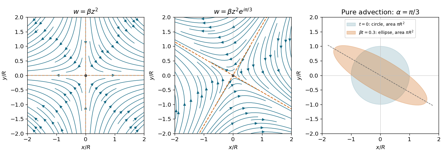
Quadratic complex potentials give hyperbolic streamlines and area-preserving dye deformation
. Original streamlines for zero phase and phase , with arrows from the analytic velocity fields. The principal extension axis rotates by . The right panel compares a unit dye circle with its image at for ; the ellipse has the same area. Details.
Taking the imaginary part of the complex potential gives the streamfunctionThe corresponding velocity field isPut . Then and . Thus the streamlines are the previous rectangular hyperbolas rotated clockwise by . Their separatrices have angles ; the extension axis is and the compression axis is perpendicular to it. The middle panel of the figure shows this rotation.
For pure advection, a marked fluid element obeysConsequently the dye circle becomes an ellipse with semiaxes and . Its area isStretching in one principal direction exactly compensates compression in the other. Equivalently the flow-map Jacobian determinant is one, as required by incompressibility. Negligible diffusion is needed to regard the sharp dye boundary as a material curve.
The coefficient of the growing term is fixed by the far-field complex potential: . On , the no-penetration boundary condition makes the cylinder a streamline, so the imaginary part of must be constant. Choosing the two terms to be complex conjugates makes that constant zero, givingThis is the zero-circulation solution, also obtained by the Milne-Thomson circle theorem. Impermeability and the leading far field alone permit an additional circulation term ; the requested algebraic form implicitly selects . No no-slip boundary condition is imposed on an inviscid flow.
The streamfunction in polar coordinates isIt gives andThe liquid still exerts normal pressure on each surface element even though tangential viscous traction is absent. For this steady flow with zero vorticity, the Bernoulli equation has one constant throughout the connected fluid region:There is no finite uniform far-field pressure to substitute for , because this straining velocity field grows with radius. Taking outward from the cylinder, the fluid force per unit axial width isIndeed while : diametrically opposite elements cancel exactly. Zero resultant force does not mean zero local pressure or zero deformation tendency.
Use the Joukowski map with , in particular its intended range . On the original circle,Define the exterior inversewhere the holomorphic square root is chosen so that at infinity. Then is the branch mapping the exterior of the ellipse to . Composition of the zero-circulation complex potential from part 4(c) with this inverse givesThe ellipse is a streamline because its inverse image is the circle, and at infinity. An additive constant in the complex potential has no effect on the velocity.
The transformed complex velocity obeys the chain rule:Since , the denominator is nonzero on and outside . The four stagnation points therefore come fromTheir physical locations areThey all lie on the ellipse, and their positions are independent of , which only sets the overall speed scale.
The printed restriction that is real and is insufficient literally: satisfies it but makes at in the exterior, so there is no exterior conformal map of the claimed type; the stated minor semiaxis would also be negative. The intended positive-parameter range, or more generally , is needed for the above solution. The reference to a sphere in the source is a wording slip: the geometry is two-dimensional flow around the mapped cylinder's elliptical cross-section.
Articles by others on the same topic
There are currently no matching articles.