Past exam of the mathematical methods II course of the University of Oxford / 2017 resit (A10289W1, CP4)

Source paper: www.whatdotheyknow.com/request/physics_preliminary_examinations/response/1162943/attach/3/Twain.7z?cookie_passthrough=1

The successive derivatives of cosine cycle through $\cos a,-\sin a,-\cos a,\sin a$. Its Taylor series about $a$ therefore separates into even and odd powers:The two brackets are the Maclaurin series of cosine and sine, givingBoth series converge absolutely for every real $x$, so regrouping the even and odd terms is valid everywhere on the real axis.

The hyperbolic cotangent isExpand the numerator and denominator using the exponential Maclaurin series:This is a Laurent series, rather than an ordinary Maclaurin series: $\coth x$ has a simple pole at zero. The printed request should be understood as the expansion obtained from the exponential series, including this unavoidable $x^{-1}$ term.

Invert the change of variables: $x=(v-u)/2$, $y=(v+u)/2$. The absolute Jacobian determinant is $1/2$, and the transformed triangle is $0\le v\le 3$, $-v\le u\le v$. HenceAt the single vertex $v=0$, the printed integrand is undefined. This causes no integral divergence: throughout the remaining triangle $-1\le u/v\le 1$, so the integrand is bounded between $e^{-1}$ and $e$. Giving the vertex any finite value, or taking a limiting integral with $v>0$, gives the same answer.

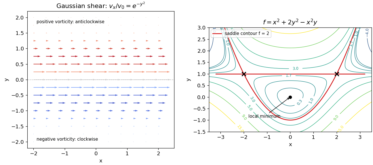
The arrows point in the positive $x$ direction, with largest speed $v_0$ on $y=0$ and rapidly decreasing length away from that line. Since only $v_x$ is nonzero,The vorticity points towards positive $z$ above the centre line and negative $z$ below it. A small fluid element therefore has local angular velocity $(\nabla \times v)/2$: anticlockwise above and clockwise below when viewed from positive $z$. At $y=0$, its speed is maximal but its local vorticity is zero. Translation speed and local rotation are different properties.

Using $r=(x,y,z)$ and constant $a$, the divergence isFor the curl, the curl of a cross product identity givesThusFor a quick sign check, taking $a=e_z$ gives $r\times a=(y,-x,0)$, whose curl is $(0,0,-2)$.

Take any differentiable curve $r(s)$ on the level surface. The chain rule givesIts tangent vector $r^{\prime }(s)$ can be any tangent direction at a regular point. Thus a nonzero gradient is orthogonal to the entire tangent plane, giving the unit normal $n=\pm \nabla f/|\nabla f|$. Nonvanishing is essential: at a critical point, the zero gradient alone does not determine a normal or guarantee a smooth level surface.

The relevant projection is the disk $x^2+y^2\le 9$. The surface area of a graph is $\iint \sqrt{1+z_x^2+z_y^2}dxdy$. Here $z_x=-2x$ and $z_y=-2y$, so polar coordinates giveThe boundary circle has zero surface area, so including the points at height zero does not change the result.

A vector line integral along an oriented parametrized curve $r(t)$ is $\int a(r(t))\cdot r^{\prime }(t)dt$; for a force field it is the work along that path. On the upper branch, set $y=t$, $x=t^2$, $0\le t\le 1$. ThensoThe stated $x$ endpoints do not distinguish the two branches of $y^2=x$. If the lower branch is intended, the same parametrization runs from $t=0$ to $t=-1$, giving instead $\boxed{4/3}$. The two values correspond to different terminal points, $(1,1)$ and $(1,-1)$; choosing a branch is necessary to make the question unambiguous.

The gradient equations are $f_x=2x(1-y)=0$ and $f_y=4y-x^2=0$. The critical points are $(0,0)$ and $(\pm 2,1)$. Their Hessian matrix isAt the origin $H=\mathrm{diag}(2,4)$ is positive definite. At either other point its determinant is $-16$, so its eigenvalues have opposite signs. ThusThe minimum value is zero and both saddle values are two. The origin is not a global minimum: at any fixed $y>1$, the term $(1-y)x^2$ makes $f$ arbitrarily negative as $|x|$ increases.

For the contour plot, the local contours around the origin are approximately $x^2+2y^2=c$. The exact saddle contour factors asso it is the union of $y=1$ and $y=x^2/2-1$, crossing at the two saddles. Other levels obey $x^2=(c-2y^2)/(1-y)$ where $y\ne 1$; the right panel of the original figure in part 3(a) shows how these branches join around the minimum and pass through the saddle contour.

The field is the gradient of $\Phi =x^2-3y^2+4z^2$ on all of ${\mathbb{R}}^3$. It is therefore a conservative vector field, and the fundamental theorem for line integrals gives ${\int }_{C}F\cdot dr=\Phi (r_{\mathrm{end}})-\Phi (r_{\mathrm{start}})$. The endpoints are $(3,0,0)$ and $(0,2,-1)$, soThe complicated intermediate path does not affect the work. Directly, $\nabla \times F=0$, consistent with the globally defined potential function.

For differentiable vector fields, expand the divergence using the Levi-Civita symbol and the product rule:The first contraction uses the cyclic identity ${ϵ}_{ijk}={ϵ}_{kij}$; the second uses ${ϵ}_{ijk}=-{ϵ}_{jik}$. This fixes the relative minus sign without guessing the orientation of the cross products.

To obtain the volume integral of a curl, test its components with an arbitrary constant vector $c$. By part (a), $\nabla \cdot (G\times c)=c\cdot (\nabla \times G)$. Applying the divergence theorem to the closed boundary, with outward unit normal $n$, givesThe last step is cyclic symmetry of the scalar triple product. Since this holds for every $c$, all vector components agree:The same regularity conditions as the divergence theorem apply: for example a continuously differentiable field on a neighbourhood of a bounded volume with piecewise smooth boundary.

For constant $b$, the curl product rule for a scalar field givesUsing part (b) and the order of the cross product,Here $dS$ inside a vector product denotes the outward vector area element $ndS$. Closedness is the condition that permits replacing the entire surface by the boundary integral of a volume.

The closed boundary includes the curved unit hemisphere and the disk at $y=0$. On the disk, $F=(0,y,0)=0$, so that contribution vanishes. On the curved part the outward normal is $n=(x,y,z)$, giving $F\times n=(yz,0,-xy)$.

Use spherical coordinates with the polar axis along positive $y$:The area element is $\sin \theta d\theta d\varphi$. ConsequentlyThis directly performs the surface integral and includes the planar cap, rather than applying the closed-surface theorem to only an open hemisphere.

The central spring extension is $x_2-x_1$. Applying Hooke's law and Newton's second law to each mass givesIn matrix form $\ddot{x}+(k/m)\left(\begin{array}{cc}1+ϵ& -ϵ\\ -ϵ& 1+ϵ\end{array}\right)x=0$. The positive off-diagonal coupling in the force equations means that displacing one mass pulls the other in the same direction.

The normal modes are the eigenvectors of the stiffness matrix. The in-phase mode has normalized vector $(1,1)/\sqrt{2}$; its central spring is unstretched. The opposite-phase mode has normalized vector $(1,-1)/\sqrt{2}$ and stretches the central spring. Their frequencies areEach mode has arbitrary amplitude and phase. Thus $x=A_{-}\cos ({\omega }_{-}t+{\varphi }_{-})(1,1)/\sqrt{2}+A_{+}\cos ({\omega }_{+}t+{\varphi }_{+})(1,-1)/\sqrt{2}$ is the general real motion. Equal coordinates belong to ${\omega }_{-}$ and opposite coordinates to ${\omega }_{+}$; the amplitudes are not fixed until initial data are supplied.

The initial vector $(d,0)$ has coefficient $d/\sqrt{2}$ in each normalized normal mode. Zero initial velocities remove their sine terms. ThereforeAt zero these give $(d,0)$ and both derivatives vanish; substitution into the coupled equations confirms the opposite signs of the two higher-frequency components.

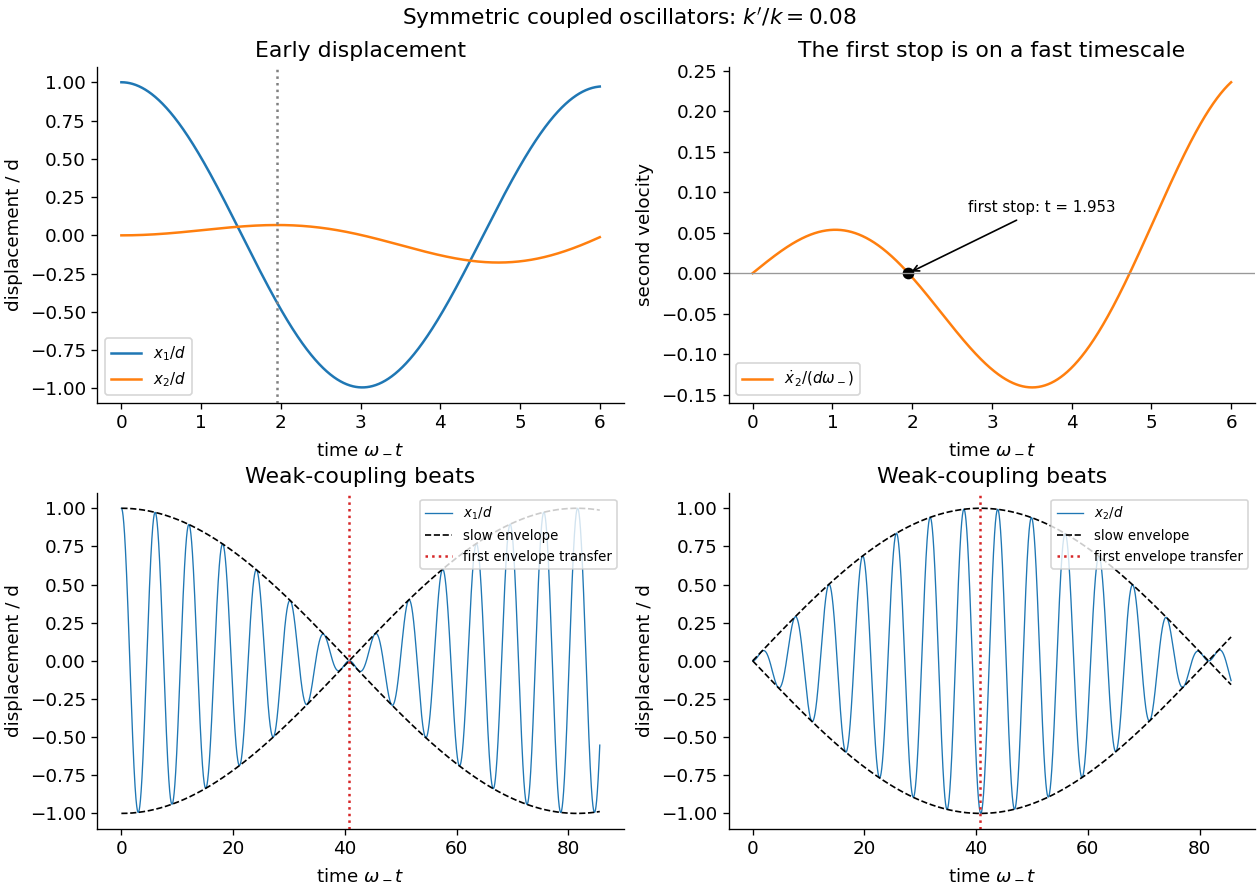
Let $\bar{\omega }=({\omega }_{+}+{\omega }_{-})/2$ and $\delta =({\omega }_{+}-{\omega }_{-})/2$. The sum and difference identities giveFor weak coupling, ${\omega }_{+}-{\omega }_{-}={\omega }_{-}ϵ+O({ϵ}^2)$, so the slow sine and cosine envelopes produce beats. The first maximum of the second envelope is at $t=\pi /({\omega }_{+}-{\omega }_{-})$, when the first envelope vanishes.

A literal first turning point of an initially stationary coupled oscillator is different from that slow envelope maximum. The first nonzero time at which the second mass is instantaneously at rest satisfiesSet $z=\bar{\omega }t$ and $\eta =\delta /\bar{\omega }\ll 1$. Dividing the derivative by $d\delta$ and expanding at $z$ of order one gives $z\cos z+\sin z+O({\eta }^2)=0$. The first positive root lies in $(\pi /2,\pi )$, where $\tan z=-z$, soThere is no earlier root: for $0<z\le \pi /2$, both terms in the exact derivative are positive when $\eta$ is sufficiently small. At the root the second displacement reaches its first local maximum. If the question instead intends the first envelope maximum, its time is $\pi /({\omega }_{+}-{\omega }_{-})\simeq \pi /(ϵ{\omega }_{-})$. That is a slow amplitude-transfer time, and is not generally a time of zero instantaneous velocity. The distinction matters because both masses keep oscillating while the envelopes change.

With $x=e^t$, the chain rule gives $x{y}^{\prime }=\dot{y}$ and $x^2{y}^{\prime \prime }=\ddot{y}-\dot{y}$. The Euler differential equation becomesIts characteristic polynomial has roots $-1\pm 2\sqrt{2}$, so, in addition to the requested transformation, its general solution is $y(x)=C_1{x}^{-1+2\sqrt{2}}+C_2{x}^{-1-2\sqrt{2}}$ on $x>0$.

Assume $v\ne 0$ so that the change of variables is invertible. The chain rule gives ${\partial }_x={\partial }_r+{\partial }_s$ and ${\partial }_t=v({\partial }_r-{\partial }_s)$. Commuting the mixed partial derivatives for a twice continuously differentiable solution givesThus the wave equation is $F_{rs}=0$. Integrating once says that $F_r$ depends only on $r$; integrating again givesThe two arbitrary twice differentiable functions are waves moving in opposite directions at speed $|v|$. This is D'Alembert's formula, on a product domain in $(r,s)$ or globally on the usual full line.

Integrating the mixed partial derivative successively gives $z=x^3{y}^2/6+A(x)+B(y)$. The first boundary value gives $A(x)=x^2-1-B(0)$. Substitution at $x=1$ then gives $B(y)-B(0)=\sin y-y^2/6$. ThereforeIts mixed derivative is $x^{2}y$, and direct evaluation checks both boundary values. Their common corner is compatible: both prescribe $z(1,0)=0$.

For two equal-amplitude waves with the same frequency and wavenumber, choose their phases so thatThe spatial amplitude and temporal oscillation separate. Positions with $\cos kx=0$ are fixed nodes of a standing wave, while positions with $|\cos kx|=1$ are antinodes. Different initial phases merely shift this pattern in space and time.

A travelling wave has a phase profile that moves at its phase velocity; a standing wave has stationary nodes and each point oscillates with its fixed local amplitude. The two counterpropagating waves carry equal opposite time-averaged energy flux, so their superposition has zero net time-averaged energy transport. Instantaneous energy can still move within the standing pattern.

For a uniform string, let $c=\sqrt{T/\mu }$. A separated mode obeys $Y^{\prime \prime }+k^{2}Y=0$, $\omega =ck$. Fixed ends require $Y(0)=Y(L)=0$, soThe first three normal modes have one, two and three half-waves respectively. Their interior nodes of a standing wave are at $x=jL/n$ for $j=1,\dots ,n-1$.

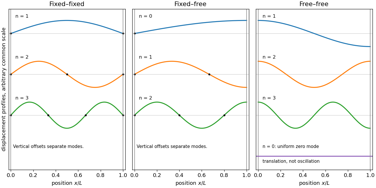
A free end has zero transverse force, hence $T{Y}^{\prime }(L)=0$, rather than zero displacement. With $Y(0)=0$, write $Y=A\sin kx$. The remaining condition is $\cos kL=0$, givingThe first three shapes have one, three and five quarter-waves. Each has a node of a standing wave at the fixed end and an antinode at the free end; the mode frequencies are in the ratio $1:3:5$.

Free ends give $Y^{\prime }(0)=Y^{\prime }(L)=0$, so the oscillatory normal modes areThere is also the zero mode $k_0=0$, with uniform displacement $y_0(x,t)=a+bt$: a free string can translate without a restoring force. It is not a positive-frequency oscillation. The first three oscillatory shapes are $\cos (\pi x/L)$, $\cos (2\pi x/L)$ and $\cos (3\pi x/L)$, with an antinode at each end. The figure includes the uniform mode too, so that the zero-frequency limit is explicit.

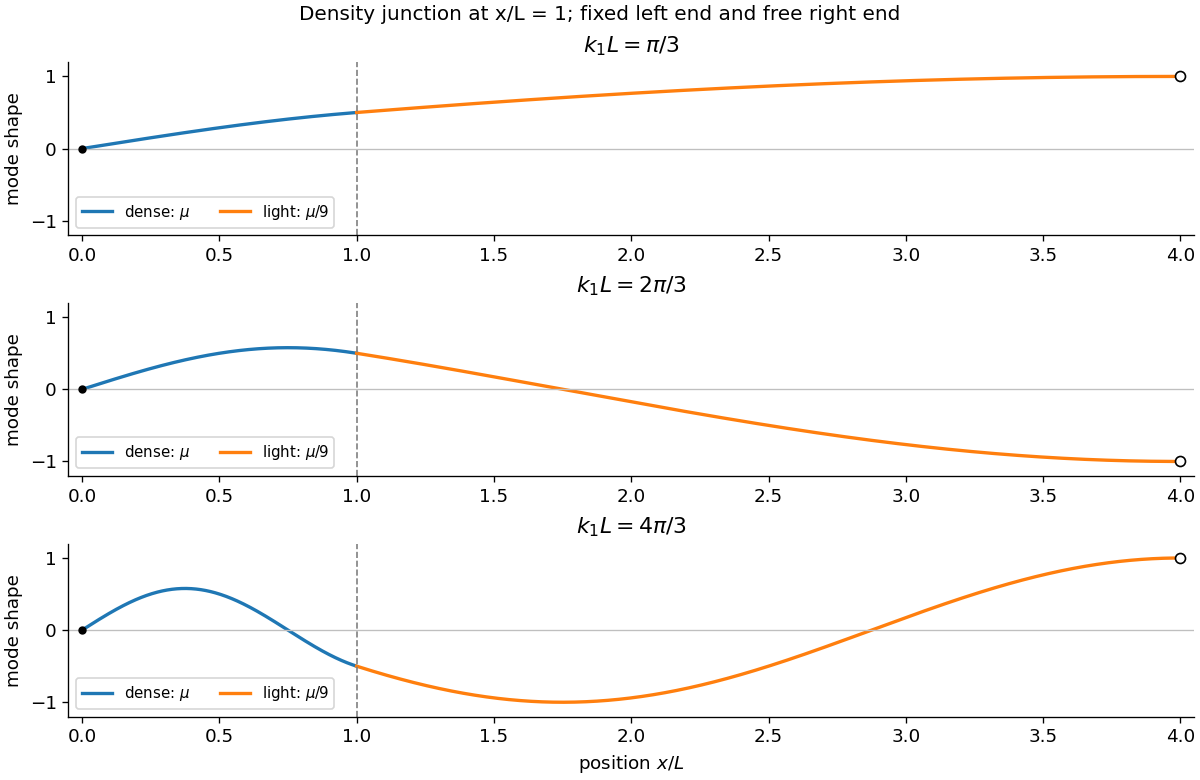
At common tension, the lighter segment has three times the wave speed, so its wavenumber at the same frequency is $k_2=k_1/3$. The fixed left end and free right end selectLet $q=k_{1}L$. Since $k_2(4L-L)=q$, continuity of displacement and of transverse force at the junction givesEqual tension makes the second condition continuity of slope. A nontrivial pair of amplitudes requires the coefficient determinant to vanish:For positive frequency, $k_2/k_1=1/3$, soNeither $\sin q=0$ nor $\cos q=0$ gives a nonzero mode, as direct substitution into the two matching equations confirms. The positive roots are $q=\pi /3+n\pi$ or $q=2\pi /3+n\pi$ for $n\ge 0$. The first modes in the figure show the changing wavelength across the junction while retaining continuous displacement and slope. The zero-frequency limit must be solved separately; the fixed and free boundary conditions allow only the trivial static solution.