The polynomial ring is an integral domain, since the product of two nonzero polynomials has nonzero leading coefficient. Let be an ideal. If , it is generated by zero. Otherwise choose a nonzero polynomial of minimum degree. For any , the polynomial division algorithm over the field gives with or . Since , minimality forces . Hence every element of is a multiple of , and . Thus is a principal ideal domain.
The nonprincipal coordinate ideal in two variables provides the contrast:If it were , then would divide and . Total degrees add when nonzero polynomials over a field are multiplied. A nonconstant divisor of consequently has degree one, its cofactor is constant, and it is a nonzero scalar multiple of . Such a polynomial cannot divide , as setting shows. Thus would be a nonzero constant and the ideal would contain one. But all elements of vanish at , so this is impossible.
For local surface coordinates and metric coefficients , affinely parametrized geodesics satisfyThese are the geodesic equation and Christoffel symbols. They follow by applying the Euler-Lagrange equation to the energy . Equivalently, in an embedded surface a constant-speed geodesic has acceleration normal to the surface.
Parameterize a circular cylinder by , where . Its induced metric is , with constant coefficients, so all Christoffel symbols vanish in this chart. ThusThese geodesics on a circular cylinder are straight generators when , circles around the cylinder when , and helices when . Constant curves arise if both vanish. For unit-speed nonconstant curves, . This description is global after allowing the angle to run through arbitrary multiples of .
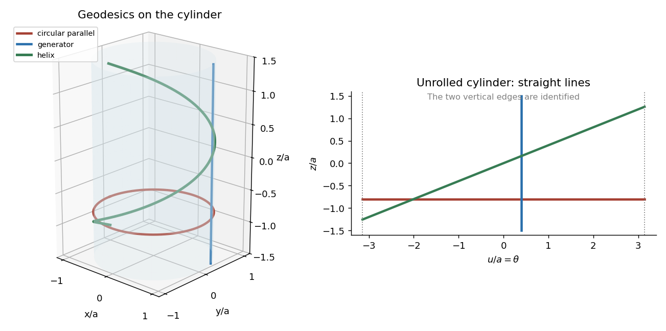
Generators, circular parallels and helices on a cylinder become straight lines when the cylinder is unrolled
. Details. 
The unrolled coordinate exhibits the intrinsic flatness of a circular cylinder: every displayed family is a straight line in . A circle is therefore a geodesic despite bending in ambient three-dimensional space; its acceleration is normal to the cylinder.
A norm is a function such that exactly when , , and . Both specified Lp norms are nonnegative, vanish only at zero and satisfy absolute homogeneity immediately from their formulas.
For the -norm, the scalar triangle inequality gives . For the -norm, Cauchy-Schwarz inequality givesTaking nonnegative square roots proves its triangle inequality. Hence both are norms.
For the sharp comparison of l1 and l2 norms, Cauchy-Schwarz yieldsThe vector attains equality, so no smaller constant works. Conversely, , giving . A standard basis vector attains equality. Thus, for ,
True. Fix a point of a nonempty connected open set and let be its path-connected component. Each point of the open set has a small Euclidean ball contained in it. A ball is convex and path-connected, so each such ball lies entirely in one path component. All path components are therefore open, and the complement of is open as well. If the complement were nonempty, these two open sets would disconnect the original set. Thus is the whole set. In fact the joining paths may be chosen polygonal.
True. For nonempty connected spaces , choose , . For each , the subspace is connected: its two connected pieces meet at . The union of these subspaces over is all of , and every piece contains the common connected subset . Their union is therefore connected. The assertion is also true if a factor is empty, since the empty product space is connected. This proves product of connected spaces.
False. The rational numbers with their subspace topology from are Hausdorff. If a subset contains two distinct rationals , choose an irrational between them; intersecting the subset with and gives a separation into two nonempty relatively open sets. Thus every nonempty connected subset of is a singleton, so it is totally disconnected. Yet no rational is isolated, because every interval around it contains another rational. Therefore is not a discrete space. Hausdorffness and total disconnectedness do not imply discreteness.
Take the circle with the usual positive, counterclockwise orientation. The only singularity is at zero, and the Laurent series givesThe coefficient of is , so the residue theorem givesThe essential singularity at zero still has a well-defined residue; the theorem does not require it to be a pole.
The integrand has simple poles at , both inside the positively oriented unit circle. At either pole , the residue is . Their sum is , so the residue theorem gives
With , the causal exponential is integrable and its Fourier transform isFor the pendulum system, a transfer function is the Fourier transform of its causal impulse response, equivalently the multiplier relating the transformed forcing to the transformed zero-initial-data response. Transforming derivatives givesPartial fractions therefore giveThe exponential transform identifies the causal response as for and zero for . It solves the homogeneous equation for , with and , the jump required by a unit impulse. The forcing is understood as switched on at zero; its transform is , and convolution with gives, if the time response is wanted,This has both stated initial values equal to zero.
Hermiticity of the Hamiltonian operator gives , soThe distinct eigenvalues force orthogonality for , and the given normalization gives one for . Therefore .
Under the time-independent Schrödinger equation, each energy component acquires its own phase:The sum converges in the state Hilbert space because the squared coefficients are summable. Orthogonality makes its squared norm at every time.
The Born rule for energy measurement givesBoth depend only on squared coefficient magnitudes, so both are time-independent. The expectation follows either by summing energy times measurement probability or by inserting the orthogonal expansion in the quadratic form of .
Normalization alone does not guarantee a finite mean for an arbitrary spectrum. The displayed energy series is finite when . Since the spectrum is bounded below by , a divergent positive tail gives an extended expectation , still independent of time; for example an abstract diagonal Hamiltonian with has this property. No growth assumption on is printed, so finiteness should not be asserted without this qualification.
Treat the four fixed row totals as four independent samples from binomial distributions. Under independence, each has the same unknown probability of a third-child boy. The pooled maximum-likelihood estimator is , so each expected cell count is . The Pearson chi-squared test of homogeneity statistic isThere are four independently varying row probabilities under the alternative, and one estimated common probability under the null; the degrees of freedom are therefore . Equivalently this is the contingency-table count. The fact that the pooled estimate happens to equal one half does not make it a specified null probability and does not change the degrees of freedom to four.
Since , reject independence at the 5% level using the stated chi-squared calibration. All expected counts are sufficiently large for the usual asymptotic test.
Write for the quantity denoted in the question, to distinguish it from the random-walk increments. Absorption at zero at time zero gives , and starting at gives . For , condition on the first step and use independence of the remaining increments. That step contributes one factor of , so the discounted gambler's ruin hitting probability satisfiesThe absorption time is finite almost surely: in each block of steps there is a probability bounded below by a positive constant of reaching a boundary by successive steps in one direction.
Trying gives , with rootsThey are positive and distinct because and . Hence the general solution is . Enforcing both boundary values givesThis includes the unbiased walk without a special limiting case, since the discount keeps the roots distinct. For uniqueness, a difference of two solutions has zero boundary values and its largest absolute value satisfies if attained in the interior. Since , .
(1) True. Over , has an eigenvalue with nonzero eigenspace . Commutativity makes invariant under : . The endomorphism has an eigenvector because its characteristic polynomial has a complex root. This is an eigenvector of both matrices, though their eigenvalues on it may differ.
(3) True. Associativity gives , so is nilpotent. A nilpotent endomorphism of an -dimensional space has index at most : in , equality at a nonzero image would make surjective on that finite-dimensional image, hence invertible there, contradicting nilpotence. Thus dimensions strictly decrease until zero, in at most steps. Therefore .
(4) False. Take on a two-dimensional vector space and . The eigenspace has dimension two, but the minimal polynomial is , in which the root zero has multiplicity one. Eigenspace dimension counts independent eigenvectors; the exponent in the minimal polynomial measures the longest corresponding Jordan chain, not that dimension.
(5) True. Factor the minimal polynomial as , with , and set . If , then satisfies , so . But also gives . Thus , so . The reverse inclusion is immediate from , proving
Use the standard commutative-ring convention with identity and a nonempty multiplicative subset. An ideal disjoint from that subset is proper. Suppose but . Maximality among disjoint ideals means that both and meet . Thus and for some , . Their product belongs to by multiplicative closure, buta contradiction. Consequently is prime. This is prime ideal avoiding a multiplicative subset.
For an integral domain, form its field of fractions from pairs with , identifying and when . Write the class as and define addition and multiplication byThe domain condition makes the equivalence relation and these operations well-defined. Every nonzero has inverse . The map is an injective ring homomorphism because implies .
For the final assertion, pass to . The image is multiplicatively closed and does not contain zero, because . Apply the allowed existence result to obtain an ideal of maximal among those disjoint from . The first proof makes prime. Its inverse image in is therefore prime, contains and avoids . The quotient is an integral domain; composeThis homomorphism kills every element of . No element of maps to zero, because the first map kills precisely and the second is injective. Thus it has both required properties. Commutativity is essential to the general statement; it is the ring convention under which the printed prime-ideal argument is used.
For a polygonal cell decomposition of the sphere, Euler characteristic givesCount incidences between faces and edges. Each edge borders two faces, and each face has at least three sides, so . If every vertex had valence at least six, counting edge endpoints would also give . Hence and , implying , contrary to Euler's formula. Thus some vertex has valence less than six.
There is a missing qualification in the printed affine-line conclusion. Two distinct parallel lines have no intersection point, so its intersection condition holds vacuously, but they do not meet at a finite point. Even three or more distinct parallel lines give the same counterexample. Consequently that conclusion is false literally without a restriction on parallel lines.
Here is the intended spherical argument when the lines are pairwise nonparallel. Lift each line in the plane to the plane through it and the origin in ; intersect these planes with the unit sphere to obtain great circles. A common axis of all these planes meets in the required common point. Suppose no such axis exists. Their circle arrangement then decomposes the sphere into polygonal faces with at least three edges. To see why a two-sided face is impossible, its two great-circle edges would have antipodal endpoints. Every defining hemisphere containing that face would contain both endpoints and would therefore have its boundary plane through their axis, contradicting the absence of a common axis.
Every circle-arrangement vertex corresponds to an intersection of lifted planes. Because no two affine lines are parallel, this axis meets , so the vertex corresponds to a finite intersection of the original lines. By the assumed multiplicity, at least three circles pass through it, giving valence at least six. This contradicts the preceding sphere count, proving concurrence in the nonparallel case. It is the ordinary vertex in a nonconcurrent great-circle arrangement argument.
Alternatively the corrected projective statement allows parallel lines, but requires the intersection condition at infinity as well, and concludes concurrence at a possibly infinite projective point. The same great-circle proof applies; concurrence at infinity represents a parallel family. The printed condition about finite affine intersections alone must not be used to assert a finite common point for such a family.
A function is Fréchet differentiable at when there is a linear map such thatThis linear map, which is unique, is the derivative .
For the chain rule, if is differentiable at and is differentiable at , then is differentiable at and . Indeed write and , where , . Since , substitution giveswhich proves the assertion, including paths on which .
For , write . Away from the two diagonal lines, and the formula is a composition of smooth functions, hence differentiable. At the origin, , so its ratio to the displacement length tends to zero. Its derivative there is therefore zero: this is quadratic damping restores differentiability at the origin.
At a nonzero point with , necessarily . Along the direction,The denominator inside the sine is locally an invertible function of , with nonzero derivative . Choose sequences tending to zero for which its reciprocal equals and . The quotients tend to and . Thus even this directional derivative fails to exist, and the function is not differentiable there. ConsequentlyFor , the formula is smooth away from zero. At zero, , so the same remainder estimate gives zero derivative. HenceNo limit of the sine factor itself is needed for either derivative at the origin.
For a nonzero holomorphic function, isolated boundary zeros produce only integrable logarithmic singularities: locally a zero of multiplicity contributes plus a bounded term. Thus the circle means below are well-defined. The identically zero function may be assigned .
1. Multiplication. The pointwise identity gives by integration, with the same extended interpretation if a factor is identically zero.
2. Zero-free normalized functions. Compactness lets us choose a slightly larger open disc on which is holomorphic and zero-free. On this simply connected disc, has a holomorphic primitive normalized by . Differentiating shows it is constant and equal to , so and is a holomorphic logarithm of . The Cauchy integral formula givesTaking real parts, using , proves . For a zero-free function with arbitrary nonzero value at zero, applying this to gives .
3. Disc factors. For ,as follows by expansion and . The denominator's possible zero is at , outside the closed disc; when it is constant. Thus the given Blaschke factor is holomorphic on a neighbourhood of the disc, has modulus one on its boundary and satisfies .
For the general formula, a nonzero entire function has finitely many zeros in the compact disc: an infinite set would have an accumulation point in a holomorphic neighbourhood and the identity theorem would make the function zero identically. List its interior zeros with multiplicities. When , divide by their factors to obtain a holomorphic function zero-free on a neighbourhood of the disc. The preceding parts give , while . Hence Jensen's formula isThe source does not explicitly rule out a zero at zero in this general step. If its order there is and with , the correct version isThus a formula using alone requires the indicated nonzero-centre assumption.
Finally, the lattice hypothesis forces quadratic exponential growth. For , all integer pairs with lie inside the disc of radius . Excluding zero, there are at least such points, and each contributes at least to Jensen's sum. Thereforefor boundary-zero-free radii, with the additional nonnegative term if needed. For all sufficiently large such radii, this is at least . Choose avoiding zero moduli and choose on each circle where is maximal. The logarithm of this circle maximum is at least the logarithmic circle mean, soThis proves lattice zeros force quadratic exponential growth; the smaller constant makes the required inequality strict.
Vary to with . The first variation of the functional isThe endpoint term vanishes. Since every smooth test variation is allowed, stationarity gives the Euler-Lagrange equation
The constant prefactor in the specified energy does not affect its stationary equation. Its integrand gives and , soTake as a screening length; for a nonzero real parameter of either sign its absolute value gives the same equation. Setting yields , henceFor and the prescribed endpoint values, the convenient hyperbolic form isIt directly satisfies both endpoint values. The energy is a positive quadratic functional, so this stationary solution is its unique minimizer for fixed endpoints: any zero-endpoint variation adds a positive quadratic energy, with the cross term zero by the equation.
In two dimensions, cylindrical area measure replaces the radial factor by . Up to an irrelevant common normalization, the corresponding energy and its modified Helmholtz equation areThus the two-dimensional radial equation is , rather than the three-dimensional equation with coefficient on the first derivative.
On a common domain where all products are defined, expansion of the operator commutator givesUse the usual quantum position and momentum operators with , the canonical commutation relation , and wavefunctions with the decay/domain conditions needed for adjoints. The cross-coordinate operators commute, soFor an eigenstate , hermiticity gives , hence its eigenvalue is real.
The product identity gives , , , . Thus the commutators with cancel, as do those with , proving . Each oscillator energy eigenspace is finite-dimensional and preserved by ; the Hermitian restriction of can be diagonalized within it. Therefore an energy eigenbasis can be chosen to diagonalize angular momentum as well.
For , differentiation gives , so . Also and , giving ; the same calculation holds for . Directly , henceThe simultaneous normalized states areTheir squared unnormalized norm is . Their inner product vanishes because the integral of is zero: the term is odd and the terms cancel by rotational symmetry.
Put . The new Hamiltonian hasFor a nonzero applied coupling , a common normalizable eigenstate would be killed by the commutator, so . It would have to be supported on the line , a set of zero planar measure, and would be the zero vector in . Thus there are no nonzero common eigenstates in this case. Merely having a nonzero commutator would not prove that conclusion for arbitrary operators; the multiplication operator here has trivial kernel. If , the original simultaneous eigenstates remain.
For the shifted two-dimensional oscillator in a uniform electric field, complete the square:Therefore and have the same shifted energyThe modified angular momentum isIt is angular momentum about the displaced centre, commutes with , and has eigenvalues on the two translated states.
Choose along the current in the inner conductor. Cylindrical symmetry and Ampère's law give for , soThe opposite current on the outer shell makes the net enclosed current zero outside both conductors; the long-cylinder approximation neglects end fields.
Take the inner conductor to be at potential above the outer. A cylindrical Gauss law surface of length encloses charge and gives . The potential difference isThus the coaxial cylindrical capacitor field and charge areThe perfectly conducting surfaces have no tangential electric field in this idealized steady model.
The Poynting vector in the annular region isIt points from the battery towards the resistor with the preceding current convention. Integrating through an annular cross-section givesThe energy is transported by the electromagnetic field in the space between the ideal conductors; the integration recovers the power dissipated at the terminating resistor.
The Euler equations for an inviscid fluid with no body force is . For irrotational flow , the identity removes the last term. Thus the gradient of is zero, giving the Unsteady Bernoulli equationThe function is spatially constant on the connected fluid region; adding a time-dependent constant to the potential changes its gauge.
For spherically symmetric incompressible radial flow, is independent of . The bubble boundary moves with the fluid, so , giving . Fix at infinity, obtaining and . The time derivative is taken at fixed , then evaluated at the moving boundary: . With pressure continuity at the interface and no capillary or viscous correction, Bernoulli gives the Rayleigh equation for an inviscid spherical bubble
The gas law and initial pressure fix . Multiply the radius equation by ; its left side is . Integrating from the zero-speed initial state gives the first integral of polytropic spherical-bubble motionTo find the permitted radii, put . The bracket becomes , nonnegative exactly for . ThereforeInitially , so the radius decreases from the upper endpoint. At the lower endpoint the gas pressure is , giving positive acceleration and an outward reversal. The first-integral zeros are simple, so the travel-time integrals near either endpoint behave as an integrable inverse square root. The bubble reaches both turning radii in finite time, and the autonomous undamped equation repeats this motion periodically. Thus the stated interval describes oscillation, rather than an irreversible approach to one endpoint.
Assume is linear, annihilates all polynomials of degree at most , is defined on the truncated-power kernels and permits interchange with the remainder integral. For , a convenient sufficient condition is that be a bounded linear functional on ; more general approximation functionals need the corresponding continuity/interchange property on their domain. Taylor's integral remainder givesApplying , the polynomial terms vanish, and the Peano kernel theorem givesHere . This is the printed raw-kernel convention; the normalized Peano kernel includes inside its definition instead, and then has no factorial outside the integral. The interchange is justified by boundedness applied to the limit of Riemann sums of the continuous kernel-valued integrand. For a kernel with , its discontinuity requires a function space/interchange assumption accommodating the step functions as well.
For the specified Simpson's rule error, direct evaluation on gives zero, so . For ,Simplifying separately on the two halves givesBoth pieces are strictly negative in the open interval; they agree at the midpoint. Their integral is , as direct polynomial integration shows. ThusThis is optimal, not merely an upper bound. For , the fourth derivative is identically one and , so the minimum constant is .
Let be shipments, with column sums eight and row sums at most the four capacities. Total demand is , below total capacity , so unused capacity is allowed. This is a transportation problem with capacity inequalities; equivalently add a dummy shop demanding four units with zero shipping cost.
Using the original PDF's cost , take the feasible solutionIts row totals are and all column totals are eight. Four units of capacity remain unused at the second factory. Its shipping cost is .
To prove that the cost is a global minimum, use the transportation dual certificate with capacity inequalities. If row potentials satisfy and , every feasible solution satisfieswhere . The second inequality uses the sign of : multiplying a capacity upper bound by a nonpositive number reverses it. Choose and . The reduced costs areso every entry is nonnegative. The lower bound is , equal to the displayed shipping cost. The minimum shipping cost is .
For the production costs in a transportation problem, add the production cost of each factory to every real shipment from that factory. Unused capacity incurs no production cost, so the dummy-shop costs remain zero. The resulting real-shop cost matrix isA feasible solution isIts row totals are and column totals remain eight, leaving four units unused at the fourth factory. Its combined cost is .
For a matching transportation dual certificate with capacity inequalities, take and . Their reduced costs areall nonnegative. The lower bound is . Thus the minimum combined production and shipping cost is , and the second allocation attains it.
Articles by others on the same topic
There are currently no matching articles.