Let . Since the kernel of a linear map and its image agree, the rank-nullity theorem gives . Thus is even. Every lies in , so . The minimal polynomial therefore divides . It cannot be , and it cannot be since ; hence the minimal polynomial is .
Choose and write using the direct sum of vector spaces . Neither component is zero: otherwise would lie in one of the zero intersections or . They are linearly independent, so is a two-dimensional vector subspace. Uniqueness of the direct-sum decomposition gives and . Also , but cannot be contained in because . Hence is one-dimensional. This constructs the required common plane for three pairwise complementary subspaces.
An ideal hyperbolic triangle has its three vertices at infinity, with sides given by geodesics. In curvature its angles are zero and its area is , using the hyperbolic triangle area formula .
To calculate the area of a hyperbolic disc, use the Poincare disc model centered at the origin. Hyperbolic radial distance is , so its Euclidean radius is . The metric area density is , givingEvery hyperbolic triangle, including ones with ideal vertices, has area at most . But . A hyperbolic triangle is geodesically convex, so if it contains a complete hyperbolic circle, it also contains the enclosed hyperbolic disc, its geodesic convex hull. This would violate the area comparison. Therefore no hyperbolic triangle contains a complete circle of radius two.
For a holomorphic function, compute its complex derivative along the real and imaginary directions. The real direction gives , while division by an imaginary increment gives . Equating real and imaginary parts proves the Cauchy-Riemann equations:For the specified real part, and . Integrating gives ; the other relation in the Cauchy-Riemann equations then forces . Thus the harmonic conjugate and the holomorphic function are
Use and metric signature . Since , the four-velocity and four-momentum areThese use the proper time and Lorentz factor; the mass shell identity is .
Initially the parent four-momentum is . By four-momentum conservation, the remaining single particle has energy and three-momentum . Applying its mass shell identity gives , henceThe positive root is selected for the rest mass; physically admissible decay data also give nonnegative remaining energy.
The divergence of this axisymmetric velocity field is . Thus it satisfies incompressibility. The apparent axis singularity in the azimuthal component is removable, since as .
Only the axial vorticity component is nonzero:The cross product is . Its components are independent of and , so its curl also has only an axial component:Meanwhile and , givingThus the required steady vorticity equation holds with . This is the balance between vortex stretching and viscous diffusion in a Burgers vortex.
Subtract the exact solution from the Jacobi method to get , hence . Convergence from every initial vector is equivalent to . If every eigenvalue has modulus below one, a Jordan block has powers that are finite sums . The polynomial factor in is dominated by geometric decay; for , the block is nilpotent. Consequently .
Conversely, for a complex eigenvector with eigenvalue , . Convergence for real errors also implies convergence for their complexification, so this tends to zero only if . Therefore the iteration converges from every starting vector if and only if , where is the spectral radius.
For the specified matrix,Its eigenvalues are , so . Hence is the convergence range. The original coefficient matrix has determinant , so the endpoints also violate its assumed nonsingularity.
An unbiased estimator satisfies for every parameter value. Under the standard full-column-rank assumption on the design matrix, the Gaussian log-likelihood for the normal linear model, up to terms independent of , is . Its maximum is the ordinary least squares minimum. Differentiating gives , and full column rank makes positive definite. ThusSince , its expectation is , proving unbiasedness. Estimating an unknown as well does not change the maximizing coefficient vector.
The printed hypotheses give but do not explicitly require full column rank. Without that condition the maximum-likelihood estimators are not unique: they are with , as in rank-deficient ordinary least squares. If , the observation distributions at and are identical. Every estimator then has the same expectation at both parameters, so no estimator can be unbiased for both entire coefficient vectors. This proves nonidentifiability prevents unbiased coefficient estimation. The stated estimator and unbiasedness claim require the usual full-rank condition.
The point is nonnegative and makes all three inequalities equalities, with objective value . To certify global optimality, combine the first upper bound with coefficient , the second with coefficient one, and the lower bound with coefficient :This is a weak duality certificate for the linear program. The feasible point attains the bound, so the optimal solution is and the maximum is . Equality forces each of the three constraints to be active; their simultaneous equations have this unique solution.
The dual space is , the vector space of all linear functionals with pointwise operations. For finite , choose a basis and define its dual basis by . Every linear functional is , and evaluation on each proves that the are linearly independent. Thus . This dimension formula is a finite-dimensional assertion.
On the space of polynomials of degree at most , define the evaluation map . Its kernel is zero: a nonzero degree-at-most- polynomial cannot have distinct roots. Since domain and codomain both have dimension , is an isomorphism. The evaluations therefore form a basis of the dual space. The linear functional has a unique expansion in that basis, proving the existence and uniqueness of the requested weights.
Explicitly, use the Lagrange interpolation polynomial basisThe differentiation weights from nodal evaluations are . If a node is zero, no singular reciprocal formula is needed: differentiate the finite product directly. For the sole weight is zero.
In a principal ideal domain, an ascending chain of ideals stabilizes: its union is an ideal , and its generator belongs to one member, which then contains the union. This proves the needed ascending chain condition. If a nonzero nonunit had no finite irreducible factorization, split it into two nonunits and select a factor that still has no such factorization. Continuing would give a strictly ascending chain of principal ideals, because with a nonunit implies . This contradicts the chain condition, so factorization exists.
An irreducible element generates a maximal ideal: any intermediate ideal is with , and irreducibility forces or to be a unit. Therefore is a prime element. In any two irreducible factorizations, the first prime factor divides a factor of the other, hence is associate to it. Cancel and continue. This proves every principal ideal domain is a unique factorization domain.
In , the multiplicative field norm is . The only units are . There is no element of norm two, so every element of norm four is irreducible: a factorization into nonunits would require norms two and two. Consequentlyis a pair of genuinely different irreducible factorizations. Neither nor is associate to .
Take the Eisenstein integers , where and . Since , the embedded subring is , whose additive index in is two. Its larger ring has Eisenstein-integer norm and is Euclidean. Indeed, write a complex quotient in the real basis and round both coordinates to integers. The coordinate errors satisfy , giving . Thus division leaves a remainder of smaller norm. A Euclidean domain is a principal ideal domain, because division by a nonzero element of least norm in an ideal leaves zero remainder. This gives the requested index-two embedding into a principal ideal domain.
Let . It is continuous and takes values in . The finite sums are continuous and their tails obeyfor every real . To prove continuity without invoking an unproved uniform-limit theorem, fix and . Choose with , then use continuity of to make near . The triangle inequality then gives . Thus is continuous; it is the scaled Takagi function .
For the general secant claim, differentiability gives , where for sufficiently small , with . Since the two endpoints straddle ,Hence the secant limit is , including cases where an endpoint equals . This proves secants straddling a differentiability point.
Now take the nested dyadic intervals , . They straddle and shrink to it. For every , and are integers, so the corresponding summand vanishes at both endpoints. For , all corners of that summand lie on the dyadic grid of mesh ; on the chosen open interval it is linear with slope . Therefore its total secant slope isRefining to the nested interval preserves the slopes of all old terms and adds exactly one new term of slope or . Thus for every , so cannot converge. This contradicts the secant consequence of differentiability at any . Therefore is nowhere differentiable. At dyadic the intervals chosen on its right satisfy the same argument. The printed reference to a denominator is naturally read as mesh , or denominator , as used here.
Suppose converges to . Continuity gives , and uniqueness of limits in a metric space gives . Hence every convergent sequence in the graph has its limit in the graph, proving is closed.
If were not continuous at , there would be and with . A compact metric space is sequentially compact, so some subsequence converges to . The closed graph then contains its product limit , forcing , contrary to the lower bound. Thus is continuous, the compact-codomain form of the closed graph theorem for compact spaces.
Take and for . Its graph is , a union of two closed sets, since multiplication is continuous. But does not tend to , so the function is not continuous.
Choose the principal branch of a multivalued function, , for . The integrand has simple poles at and a branch cut along the negative real axis. Its residues arewhose sum is .
For , close the Bromwich contour to the left using a rectangle with outer real part and horizontal edges at imaginary parts , indenting the cut and zero. On every distant edge, , and . Each edge has length and , so its integral is . The small circle of radius about zero contributes . The tails of the original vertical integral are absolutely bounded by as well.
On the upper and lower banks at , the square roots are and , respectively. With the upper bank traversed toward zero and the lower bank away from zero, their combined integral isThe cut integral converges near zero since is integrable, and at infinity by exponential decay. The residue theorem, followed by and , therefore givesFor , close the Bromwich contour to the right. There are no enclosed poles or cuts, and there. The same distant-edge estimates show for .
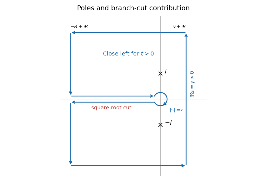
Left-closing Bromwich contour with the principal square-root cut, two pole residues, and a small indentation at zero
. Details. 
For the large- expansion, . Scaling and using the given integral yields . Integration by parts twice gives the next coefficient . The remainder is bounded by . Thus, without needing a globally convergent termwise integration of the local power series,In particular, the requested two leading terms are , interpreted as an additive asymptotic expansion. This is Bromwich inversion with a square-root branch cut.
Write with . Substitution into the ordinary differential equation givesUnless the series terminates, its coefficient ratio is , so it converges for every finite . A coefficient first vanishes exactly when is a nonnegative integer , and then , . Thus is a polynomial precisely for , in which caseis the normalized Laguerre polynomial.
Multiplying the differential equation by gives . Multiply by , subtract the equation with the indices exchanged, and integrate over . The boundary term vanishes both at zero and infinity. ThereforeThis is the weighted orthogonality of the Laguerre polynomials.
Their leading coefficients show . Since have distinct degrees, they form a basis of that polynomial space. Hence , and comparison of leading coefficients gives . Likewise the degrees of and for run through and , respectively. A nontrivial linear combination cannot cancel its highest-degree term, so these functions are linearly independent.
For , this gives the basis of the cubic polynomial space, establishing the specified expansion. Its weighted integral is : integrates to one, and are orthogonal to , and integrates to zero. At the two roots of , the expansion reduces to . Solving these two equations for givesFor explicit verification, the recurrence gives , . Thus , are distinct positive roots and , . This is the two-node Gauss-Laguerre quadrature rule, exact for every cubic.
The parity operator acts by . For an even potential, differentiating twice and using proves on the parity-invariant domain of the Hamiltonian operator. Therefore each energy eigenspace is invariant under . The projectors and split it into even and odd subspaces, giving a basis of simultaneous eigenstates. An odd state obeys , hence .
The infinite walls impose , with the wavefunction zero outside. It is continuous at the central delta potential. Integrate the stationary Schrödinger equation over ; the energy integral tends to zero and the Dirac delta function contributes . This givesFor the given piecewise positive-energy form, . Replacing by swaps the two pieces and leaves their values unchanged, proving . The value at zero is , and the one-sided derivatives are and . The jump condition gives . The wall at gives , henceFor the undivided wall equation instead gives the usual free even roots. For , set and . In every interval there is exactly one root: writing gives , whose two sides are respectively strictly decreasing and increasing. These are all positive even roots; the quadratic form is nonnegative, so there are no negative eigenvalues. Thus and .
The printed limit of this absolute energy difference is false. The exact quantization equation gives , so but . ConsequentlyThus the high-energy shift from a central delta barrier is a finite positive constant, not zero. The corrected vanishing statement is the relative shift , or the wave-number difference . Physically, highly energetic particles are weakly affected in relative terms by a fixed point barrier. The free even wavefunction normalized in has density at the origin, so the barrier's first-order expectation is , matching the exact limit.
Odd states vanish at zero, so the delta term and the derivative jump both vanish. Their normalized wavefunctions and energies arewith zero wavefunction outside. They do not depend on . These even and odd sectors describe the central delta barrier in a symmetric infinite well.
In electrostatic equilibrium, the electric field inside a perfect conductor is zero. Apply the Faraday's law to a thin rectangular loop crossing the surface, with its long sides tangential and its short sides shrinking to zero. It yields continuity of the tangential electric field. Since its interior value is zero, . Earthing fixes the electric potential at the plane to zero. For completeness, a thin Gauss law pillbox gives ; the normal component can be nonzero because of induced surface charge. These are the electrostatic boundary conditions at a conductor.
The charge and its proposed image charge give the exterior electric potentialAt the terms cancel, so everywhere on the plane and its tangential derivatives vanish. Thus the image construction satisfies the earthed-conductor boundary conditions. It has the correct point-charge singularity, is harmonic elsewhere in , and decays at infinity; electrostatic uniqueness identifies it with the exterior solution.
At instantaneous height , the image charge is a distance below the real charge, giving force with . Multiplying by and using rest at givesThe induced-conductor potential energy is , not the full energy of a pair of independently movable charges. On the falling branch, integrate the reciprocal speed:The last integral is by . Hence the fall time of a charge toward a grounded plane in the electrostatic Newtonian model isFor there is no force and the particle remains at rest.
Use the steady inviscid, hydrostatic, slowly varying channel approximation, without a hydraulic jump. Conservation of volume flux per unit width gives . The free-surface Bernoulli equation isDividing by yieldsThe parameter here is the squared upstream Froude number. For nonzero discharge, regarding as a function of , its derivative is . It has its unique maximum at , where the local Froude number is one. Substitution gives . This maximum is the hydraulic control over a smooth hump.
The upstream flow is subcritical flow, with . On this branch , so the depth decreases as the bed rises; the velocity increases. Since the crest height is below , the depth remains above and never becomes critical. Over the falling side of the hump the depth increases again to downstream. The free surface falls over the hump: on the subcritical branch.
The upstream flow is supercritical flow, with . Now , so the depth increases over the rising hump and the velocity decreases, while the free surface rises. Since , the depth stays below . On the descending bed it decreases back to downstream, remaining supercritical throughout.
At the crest the two depth branches meet at . For a smooth nondegenerate maximum of the bed, is proportional to , while expansion of the depth relation gives . A differentiable flow through the crest therefore switches branches rather than following the cusp obtained by staying on the same branch. Subcritical upstream flow becomes supercritical downstream; supercritical upstream flow becomes subcritical downstream.
When and the bed returns to zero, put . The head equation becomes , orThe root is the original subcritical branch. The other positive root is smaller and lies on the supercritical branch, givingThis is the smooth transcritical, shock-free solution. A downstream hydraulic jump would require further downstream conditions and energy loss. A degenerate flat crest can also require a branch-selection condition; the standard critical-control interpretation uses a nondegenerate smooth crest. For , , so a positive hump is incompatible with the prescribed upstream critical head. If , the head equation is the still-water relation ; a crest of height dries out, so the wet transcritical-flow interpretation requires .
A critical region is the set of sample outcomes on which a test rejects its null hypothesis. Its power function is ; its size of a statistical test is . Randomized tests replace the indicator of by a rejection probability .
The Neyman-Pearson lemma states that for two simple hypotheses with densities , the test that is one where , zero where , and randomized on equality to have null rejection probability , maximizes power among tests of size at most . Here . To prove it, let be any competing test. Pointwise, , since both factors have the same sign off the equality set. Integrating givesThis proves the lemma, including equality-set randomization and points where .
Take the exponential parameter to be its rate: for . For , the joint likelihood ratio is , decreasing in . Hence for the most powerful test isThere is no boundary randomization because has a continuous gamma distribution. Its density follows by repeated convolution: . Integrating by parts gives the exponential-rate likelihood-ratio test powerThe threshold is the unique positive solution of this formula at with value . Differentiating the finite sum yieldsThus the power function is strictly increasing, and its supremum over is . Therefore the same test has size for the composite null . Since the threshold does not depend on the particular larger rate, it is also uniformly most powerful against all . The endpoint sizes zero and one have their trivial constant tests.
Read the maze as two four-cycles: outer vertices , inner vertices for modulo four, edges , , and , together with edges from every to the target . The starting vertex is an outer vertex. Outer degrees are three and inner degrees are four.
For the ordinary random walk on a graph, symmetry gives a common expected hitting time from an outer vertex and from an inner one. First-step conditioning givesThus and , yielding and the requested starting mean moves.
For the non-backtracking random walk, the current vertex alone does not form a Markov chain. Use states recording previous and current vertices. Before hitting , its transitions are with probability for each neighbor . Add a starting state with no preceding vertex, choosing its first neighbor with probability , and an absorbing hit state. This specifies the full Markov chain.
Its directed edges aggregate into types , determined by the two vertex layers. From the next type is or with probability each. From it is with probability and the absorbing state with probability . From it is always . From it is , or the absorbing state with probability each. Every nonabsorbing type has a positive uniformly bounded chance of hitting within at most three more moves, so its mean time is finite.
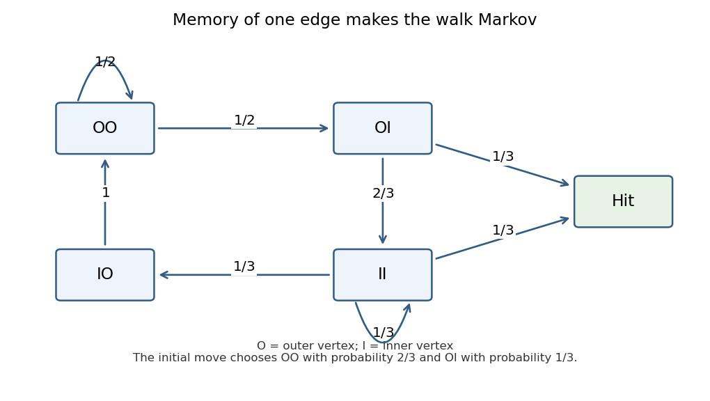
Transition probabilities between the four directed-edge types of the non-backtracking maze walk and its absorbing target
. Details. 
Let their remaining mean times be in that order. The first-step equations areSolving gives , , , . The first move from the initial outer vertex reaches type with probability and type with probability , so the intelligent starting mean isThis hitting a hub from two four-cycles calculation reduces the mean from to , saving moves. Excluding immediate reversal removes wasteful two-step returns, although it does not guarantee that the next move is toward the target.
The monomials with and form a basis of the given vector space. There are of total degree , soOn that basis the linear operator is diagonal:Both summands of the eigenvalue are nonnegative integers. Their sum is zero precisely when . Thus the kernel is the span of those members of whose total degree is at most . In particular it is for and for ; for it is the constants. The image of a linear map is the span of all the other permitted monomials, since each has a nonzero diagonal eigenvalue and hence is the image of its reciprocal multiple. No excluded monomial can occur in an image because its diagonal coefficient is zero.
The trace is the sum of these eigenvalues. At degrees zero and one all contributions vanish. At degree two the contributions are , summing to four; at degree three they are , summing to sixteen; at degree four they are , summing to forty. ThereforeThis is the diagonal monomial action of a second-order Euler operator.
For a finite group of order with prime and , the Sylow theorems assert that a subgroup of order exists; every subgroup whose order is a power of is contained in one such Sylow subgroup; all Sylow subgroups for that prime are conjugate; and their number divides and is congruent to one modulo . A unique Sylow subgroup is a normal subgroup, since conjugation cannot move it to another one.
Here , so divides eight and is congruent to one modulo seven. Hence or . In the first case the Sylow subgroup of order seven is normal. In the second case, any two distinct order-seven subgroups intersect only at the identity, because a nontrivial intersection would generate both prime-order subgroups. Their nonidentity elements therefore account for elements.
Exactly eight elements of the group remain. Every Sylow subgroup of order eight consists entirely of these remaining elements: a nonidentity element in it has order a power of two and cannot be one of the order-seven elements already counted. Each such Sylow subgroup must consequently equal the remaining eight-element set. It is unique and hence normal. Thus a group of order 56 has a normal subgroup of order seven or of order eight.
The contraction mapping theorem states that a contraction mapping on a nonempty complete metric space has a unique fixed point. Here contraction means that some satisfies for all .
For a proof, choose and iterate . Induction gives . For , the triangle inequality and a geometric series giveThus the iterates form a Cauchy sequence, and completeness supplies a limit . A contraction mapping is continuous, so . If is another fixed point, , forcing . This proves existence and uniqueness.
For the exponential problem, use on the complete metric space . Its derivative isPutting , the function has maximum at , as its derivative is . By the mean value theorem, , so is a contraction mapping on all of . Let be its unique fixed point. The compositions commute, so ; uniqueness of the fixed point of forces . Conversely every fixed point of is fixed by . Hence there is exactly one real solution of . It lies in because and then . This uses the iterated contraction argument without claiming that itself contracts on all of .
A Hausdorff space is a topological space in which any two distinct points have disjoint open neighborhoods. Let be a compact subset of a Hausdorff space and . For each , choose disjoint open neighborhoods of and of . The cover , so compactness gives a finite subcover . Their paired intersection is an open neighborhood of disjoint from . Thus every point of its complement has an open neighborhood in the complement, proving every compact subset of a Hausdorff space is closed. The empty set case is immediate.
In the cocountable topology on an uncountable set, any two nonempty open sets intersect: their combined complements are countable and cannot exhaust . Thus the space is not Hausdorff.
Nevertheless every compact subset is closed here. In fact only finite subsets are compact. To prove this, suppose is infinite and choose distinct points . The open setsform an increasing open cover of , and hence of . Any finite selection is contained in for its largest index , which misses . So is not compact. Finite sets are compact in any topological space, and in this cocountable topology they are closed because their complements are open. This proves the claimed behavior of compact subsets of a cocountable space.
The Fourier sine series coefficients of on areby integration by parts. The odd periodic extension is piecewise smooth, so the Fourier series converges to at every interior point. HenceTo justify integration from zero, the Fourier sine series partial sums converge to in L2 norm. By the Cauchy-Schwarz inequality, integration from zero to any has error at most times that L2 norm error, uniformly in . Integrating the partial sums and taking the limit therefore givesThe integrated series is absolutely and uniformly convergent, since its terms are bounded by . Thus the resulting Fourier cosine series hasIndependently, the constant coefficient isComparison yields the requested exact sum
In SI units, Gauss's law relates the outward electric flux through a closed surface to its enclosed charge:The outward unit normal specifies the sign of the electric flux.
The uniform charge density is . Spherical symmetry makes the electric field radial and constant in magnitude on each concentric sphere. A sphere of radius encloses charge . Gauss's law therefore gives , soThis also defines the zero electric field at the centre by continuity.
Take the upper hemisphere to have . Integrate the force using the total interior electric field from part (a). This computes the net external force on the upper hemisphere, since the forces between pairs of its own charge elements cancel by antisymmetry of the Coulomb force. Horizontal components cancel by symmetry. The vertical component isA horizontal section at height has area , soThus the lower hemisphere repels the upper one vertically upward, withThe result is the same for either sign of , as expected for the force between hemispheres of a uniformly charged ball.
For a standard collinear Lorentz transformation, put and , with . Then and . Define the rapidity . The identities and , with , give and . Substitution proves the desired hyperbolic form.
Adding and subtracting those transformed coordinates uses and yieldsA second collinear Lorentz transformation of rapidity multiplies these two null coordinates by and . Their total factors are therefore and , provingThe hyperbolic tangent addition formula now gives the velocity composition lawAll velocities here are signed along the same axis; the speed is the absolute value if either frame moves in the opposite direction.
Use the ideal steady incompressible-flow model, neglecting height change across the smooth nozzle. Flow conservation gives inlet and outlet speeds and . Set atmospheric pressure to zero. The Bernoulli equation between inlet and outlet givesChoose a control volume containing the fluid in the nozzle, with the positive axis pointing toward the outlet. The integral momentum equation givesThus the fluid's force on the nozzle is , in the outlet direction. Substitute the pressure and velocities:The fireman's holding force is equal and opposite. Therefore the required force points upstream and has magnitudeThis is the holding force on a contracting nozzle; retaining the inlet pressure force is essential to its sign and value.
Label the towns from left to right, and the treatment plants as upper-left, upper-right, lower-left and lower-right. Model each treatment capacity as a sink arc to the sea. Incoming untreated sewage can be forwarded, so the numbers inside the plant circles constrain treatment, not total throughput.
The sum of treatment capacities is , so no feasible flow network can handle more than 62. Here is a feasible routing attaining that upper bound. Send town inflowsEvery town-to-plant flow respects its directed pipe capacity. Send an additional five units from to through their bidirectional pipe, whose capacity is twelve, and two from to through their bidirectional pipe, whose capacity is fourteen. Use neither horizontal plant-to-plant pipe.
Now receives and treats all of it. Plant receives , forwards five and treats fourteen. Plant receives and treats all of it. Plant receives , forwards two and treats twelve. Thus flow conservation holds at every plant and all treatment capacities are saturated. The routing proves the upper bound is achievable:This is one optimal assignment, not a uniqueness assertion. The total bound comes from the cut consisting of all treatment-to-sea arcs; the explicit routing supplies a matching maximum flow certificate.
The ascending chain must stabilize because is finite-dimensional. Once , it stays stable: if , then , so ; induction repeats the argument. Choose a positive such , giving .
If , write . Then , so and . By the rank-nullity theorem, the dimensions of those two subspaces sum to . HenceThis proves the finite-dimensional form of the Fitting lemma.
If , the kernel contains a nonzero vector , and is a proper vector subspace. Extend a basis of that image of a linear map to a basis of and choose a nonzero linear functional which vanishes on the former basis. Define . It is a nonzero endomorphism, since takes a nonzero value somewhere, andThus a singular endomorphism has a nonzero two-sided annihilator, as required.
For an idempotent linear map , the decomposition shows : the first term is killed by , the second is fixed, and a vector both fixed and killed is zero. An adapted basis makes its matrix , with . Consequently equal ranks give identical adapted matrices and therefore a change of basis relating . Conversely, similar matrices have the same rank because pre- and postmultiplication by invertible matrices preserve rank. Hence and are similar exactly when their ranks agree, proving the similarity classification of idempotent linear maps.
The centre of a group is . It is a normal subgroup. For with , let act on itself by conjugation. The orbit-stabilizer theorem makes the size of the conjugacy class of equal to , a power of . A class has size one exactly when ; every other class size is divisible by . The class equation therefore givesso divides . Since the identity belongs to the centre of a group, its size is a positive multiple of . This proves the nontrivial center of a finite p-group.
If is cyclic, choose a representative of a generator. Every element is for an integer and . Any two such elements commute, since their central factors commute with everything and their remaining factors are powers of the same element. Thus is an abelian group, , and the cyclic quotient by the centre of a group is trivial.
For a non-abelian group of order , the centre of a group has order , or by the proved result and Lagrange's theorem. The last would make the group abelian. The middle would make have prime order and hence cyclic, also making abelian by the preceding argument. Therefore its centre has order .
Finally write the given upper-unitriangular matrix as . Direct matrix multiplication givesIt commutes with every exactly when for all . Taking forces , and taking forces ; those conditions also suffice. Thus the centre of a group in this Heisenberg group over a prime field is
For stereographic projection, choose the north pole of the unit sphere and identify the plane with the complex plane by . Project a point along the line joining it to ; adjoin for the north pole to identify the whole sphere with the Riemann sphere. A point of that line is . Its last coordinate vanishes when , givingUsing , or solving this line's second intersection with the sphere, gives the inverseA great circle lies in a plane through the origin. Its projected equation isIt is a straight line only if , meaning the plane contains the north pole and the south pole. Thus if all three sides of a nondegenerate spherical triangle projected to straight sides of a Euclidean triangle, all three distinct side planes would contain both poles. Each pair of side planes could then meet on the sphere only at those same two poles, which cannot supply three distinct triangle vertices. A nondegenerate spherical triangle cannot project to a Euclidean triangle. If a side passes through the projection pole, its image is unbounded and also cannot be a finite triangle side.
A nonidentity rotation in three dimensions has an axis through the origin: an orthogonal three-by-three matrix of determinant one has an eigenvalue one, since nonreal eigenvalues pair as conjugates, real eigenvalues are , and their product is one. Its axis meets the unit sphere in an antipodal pair, which is fixed. In the identity case every point is fixed, so an antipodal pair can again be selected. Projecting and giveswhenever both points are finite. Thus the associated Möbius transformation fixes an antipodal pair satisfying the claimed relation. The universally valid relation is on the Riemann sphere, with and paired. A rotation about the projection axis fixes exactly that pair, so the PDF's literal finite product needs this extended-coordinate convention. This is the antipodal stereographic coordinate relation.
TakeIts defining matrix has nonzero determinant eight, so it is a Möbius transformation. Direct substitution shows that it fixes and , which satisfy . However, . Differentiating the inverse projection formula gives the round spherical line element . At a fixed finite point, its local length multiplier under a Möbius transformation is exactly , since the metric factors in numerator and denominator agree. Here that multiplier is two, so this map is not an isometry and cannot be a rotation in three dimensions of the sphere. It demonstrates that antipodal fixed points do not characterize sphere rotations.
Reflection of the sphere in the plane sends to . It preserves dot products, hence the spherical distance between every pair of points. Its stereographic expression isThis is an isometry of the sphere but is not a Möbius transformation: at any finite point, its complex difference quotient is one along real increments and minus one along imaginary increments, so it is not holomorphic. A Möbius transformation is holomorphic away from its pole. The geometric distinction is that this reflection reverses orientation, whereas a Möbius transformation preserves it.
A subset is an open set when every has some radius for which . If a continuous function takes only the values zero and one, continuity at with tolerance gives a neighborhood on which . The two possible values differ by one, so throughout that neighborhood. Thus is locally constant, and the zero linear map is its derivative, since the difference is exactly zero for all sufficiently small . Hence everywhere.
For the bound on , parametrize the segment by , . The chain rule givesby the definition of operator norm. The mean value theorem applied to the real function provesIf the endpoints agree the estimate is immediate. No continuity of the derivative is required.
For the finite-line complement, each removed line is closed, so is open. Because , there is a unique affine plane containing and , and a unique affine plane containing and . Choose outside the union of these finitely many planes, using the permitted fact about finite plane covers. In particular . If met at a point , then , and the line through lies in . Since is on that same line, it would belong to , a contradiction. The same argument using applies to . Thus and can be joined in by these two segments, proving polygonal connectivity of a finite-line complement.
Finally a continuous has zero derivative by the first argument. Apply the proved segment estimate with separately on and . It gives . Since were arbitrary, is constant on .
For the Joukowski map , the derivative is . Thus it is a conformal map at every finite except its pole at zero and its critical pointsThe pole maps to ; as a map of Riemann spheres it is a simple pole and is not a branch point. Neither is the point at infinity, where the map behaves like .
An appropriate domain is the upper exterior half-discFor , on . To prove surjectivity and injectivity, solve as . Its two roots have product . For , neither root lies on the real axis or on , since either boundary maps to the real axis. Exactly one root therefore has modulus greater than . The imaginary-part identity forces that root to have positive imaginary part. It is the unique root in , so maps conformally and bijectively onto the upper half-plane.
HereThis entire function vanishes exactly at , , and those points map to . The second derivative there is , so each is a simple critical point of the conformal map:Take the half-stripWriting , its imaginary part maps to . More precisely, maps bijectively onto , with inverse using arguments in . ThenPart (i) with , followed by positive real scaling, proves that this second map is a conformal bijection onto the upper half-plane. Their composition proves the required result and gives the half-strip conformal map by hyperbolic cosine.
For small transverse displacement, the wave equation on a string iswhere is the tension and is mass per unit length. Using separation of variables, put , the ratios equal a constant. The fixed-end conditions exclude nontrivial solutions for nonnegative separation constants; for they give and , . The associated angular frequencies are . Thus the general superposition of separated normal modes isThe string is initially straight and at rest before the impulse, so . Assume the hammer interval lies inside . The imposed velocity has Fourier sine series coefficientTherefore , giving the amplitude of every excited normal mode.
The string energy is . At the impulse it is . Orthogonality of the sine modes gives initially; each mode subsequently exchanges kinetic and elastic energy while retaining that total. Thus the modal energy of a localized velocity impulse on a string has fractionsFor and , a mode is absent exactly when or . Hence the unexcited modes are precisely
Articles were limited to the first 100 out of 214 total.
Articles by others on the same topic
There are currently no matching articles.