Use azimuth measured from north toward west, and positive hour angle westward. These conventions are forced by the signs in the coordinate formulae. In the diagram the observer is at , the local vertical meets the celestial sphere at the zenith , and the north celestial pole is . The astronomical horizon is perpendicular to ; the celestial equator is perpendicular to . Their intersections with the celestial meridian give the north horizon point and the upper equatorial meridian point.
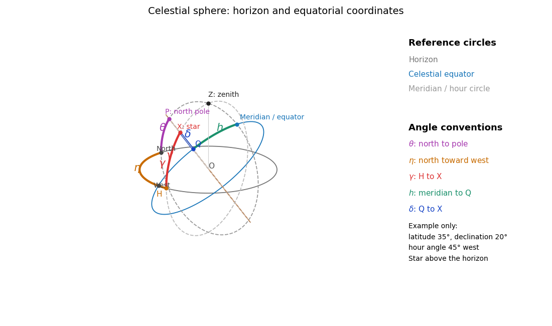
The celestial sphere with horizon and equatorial coordinates
. Details. The north celestial pole has altitude ; thus the angle between and is . Project along its vertical great circle onto the astronomical horizon at : the arc is the altitude , and the westward horizon arc from north to is the azimuth . Project along its hour circle onto the celestial equator at : the arc is the declination , and the westward equatorial arc from the upper celestial meridian to is the hour angle . Equivalently the triangle on the celestial sphere has sides , and . All five angles refer to arcs on their specified reference circles, not arbitrary angles in the projected drawing.
Let be orthonormal unit vectors north, west and upward. A direction of altitude and westward azimuth isThe north celestial pole and the upper equatorial meridian direction areIn the equatorial coordinate system, the same unit vector is . Taking dot products with respectively givesThis is an orthogonal transformation between two bases, so it preserves the length of the direction vector. Recover from both its sine and cosine to keep the correct quadrant. At the zenith, azimuth itself is undefined; the vector equations remain meaningful by continuity. Using the more usual eastward azimuth changes the sign of the second equation.
Local sidereal time is the right ascension on the upper celestial meridian. Since right ascension increases eastward while hour angle increases westward, their difference isOne hour of either coordinate is . For a fixed stellar direction, increases at the sidereal rotation rate. Mean sidereal time should be used with mean right ascension, or apparent sidereal time with apparent right ascension, for the same reference equinox.
Write for one sidereal day in minutes and . An equatorial star at an equatorial site rises along a vertical great circle, passes through the zenith, and descends on the opposite side. Its azimuth changes by at the crossing. The restricted altitude travel prevents following it continuously by rotating over the zenith.
The maximum azimuth rate is radians per minute, so the shortest half-turn takes minutes. During that lost-track interval the star moves throughFor minutes this is approximately ; using a 24-hour day gives . If the quoted zenith blind spot size means the angular radius of a symmetrically placed crossing gap, it is , approximately .
This derives the ideal crossing-gap size with instantaneous acceleration and an available altitude drive. It does not uniquely define a circular forbidden region for all nearby trajectories. For example, at an equatorial site a star of small nonzero declination has maximum azimuth rate at transit: its minimum offset is constrained by . That rate contour and the half-turn crossing gap are different definitions of a zenith blind spot. Actual tracking footprints also depend on acceleration and the reacquisition strategy, as discussed in the telescope designers' tracking discussion.
A star of declination crosses the zenith. Its direction rotates around the celestial pole at , but its actual angular velocity on the celestial sphere is . Consequently the small-angle crossing-gap estimate becomesFor clarity, the factor is the radius of the star's daily circle on a unit celestial sphere; it does not modify the sidereal hour angle rate.
The estimate assumes the required slew is nearly . A more exact ideal symmetric reacquisition calculation is possible. Let the endpoints have hour angles and suppose , small enough that both endpoints are above the astronomical horizon. The horizontal direction components are and . Their shortest azimuth separation isThe minimum ideal gap satisfies ; its angular separation is . Expanding for a fast drive gives the boxed expression. At an equatorial site exactly. At a geographic pole the direction with is stationary, so the crossing argument is inapplicable and the limit is zero. A full near-zenith rate-limited footprint still requires specifying the trajectory and drive model.
For thin contacting components, optical powers add. At wavelength the total optical power is . An achromatic lens has , henceFor normally dispersive optical glasses, both index differences are positive, so the two components have opposite curvature factors and opposite optical powers. This uses the thin Lensmaker's equation; finite thickness and separated principal planes require a more detailed design. If the denominator vanishes, use the undivided power-balance equation rather than this ratio. Two-wavelength correction alone does not eliminate the residual chromatic aberration at every intermediate wavelength.
At the line, the focal lengths obey . ThusRearranging givesThe last equality uses the Abbe number definition. The minus sign signifies a converging and a diverging component, with the normal optical glass convention and nonzero finite focal lengths.
Set and . The achromatic doublet power balance gives two linear equations:For distinct nonzero Abbe numbers, solving yields and , and thereforeEqual Abbe numbers force the total optical power to vanish under the achromatic condition; they cannot give a nonzero-power thin achromatic lens. Closely matched Abbe numbers require large opposing component powers and are generally unattractive because of the resulting sensitivity and other optical aberrations.
is the Abbe number, a dimensionless inverse measure of optical dispersion. Large means weak dispersion. The Abbe diagram below spans a representative visible-light optical glass range, roughly and . The shaded families are schematic, not exact catalogue boundaries; modern compositions overlap and include high-index crown glasses.
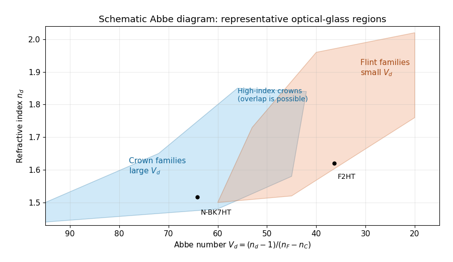
An Abbe diagram of representative optical glasses
. Details. For a usual positive objective, choose component 1 as a higher- crown glass and component 2 as a lower- flint glass. Then , , and : the crown glass is converging, the flint glass diverging, and their dispersive powers cancel while leaving positive net power. The Abbe numbers alone do not set their absolute focal lengths; the specified total focal length does. As a representative pair, , gives , . Representative index and dispersion data are given in SCHOTT's optical-glass data.
The optical telescope focuses the sky onto an optical slit; the collimator turns the selected light into a beam incident on the reflection diffraction grating; the optical camera images each diffracted direction onto the photodetector. The drawing also shows the monochromatic optical slit image for uniform optical slit illumination in the geometric, slit-limited approximation.
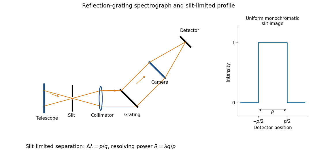
Reflection-grating spectrograph and slit-limited line profile
. Details. Near the chosen wavelength , a small wavelength increment moves the image by , where is the magnitude of the linear spectral dispersion. An optical slit image of physical width therefore has an apparent spectral width . With one optical slit width as the adopted separation criterion,Uniform illumination gives a top-hat monochromatic profile of width ; an unresolved stellar image need not illuminate the optical slit uniformly, so its profile follows the actual illumination convolved with the instrument response. Negligible optical slit diffraction and optical camera optical aberrations do not remove the finite diffraction grating diffraction width. The formula is the slit-limited result when that width is small compared with , rather than a universal exact line-profile criterion.
Let be the optical telescope focal length, the physical optical slit width, the collimator focal length, and the incident collimated beam diameter. For the grating equation , differentiation at fixed wavelength gives . Thus the monochromatic optical slit image width isThe incident and emergent optical pupil widths are and . Multiplying cancels the anamorphic magnification of a grating:This is conservation of the Lagrange optical invariant in the dispersion plane. It uses paraxial optical slit angles, an unvignetted optical pupil and matching full-width conventions for .
Insert the slit-limited spectral resolving power into the invariant expression:Here is a magnitude; a signed linear spectral dispersion would require the corresponding absolute value. Since has units of photodetector length per unit wavelength, has units of length.
Differentiate the grating equation with incidence fixed:The second formula is local to a spectrum centered on the optical camera optical axis, where to first order. Since the illuminated surface width projects to optical camera beam width ,The expression takes positive diffraction order and width magnitudes. Off-axis, a photodetector mapping also has a factor; the exam's compact formula uses the local paraxial mapping.
Substitution of givesThe incident and outgoing optical path length contributions between the two ends of the illuminated diffraction grating add. Their total is , so is the edge-to-edge optical path difference in the selected diffracted direction. This is a length, not a dimensionless resolving power. With illuminated grooves, and the ideal diffraction grating diffraction-limited spectral resolving power is . A wide optical slit generally gives a smaller slit-limited ; this distinction limits how far the slit-width scaling may be extrapolated. All of these formulae assume the stated reflection-grating sign convention.
The number of spaxels is . To obtain definite scaling exponents, keep the spectral resolving power, wavelength interval, diffraction grating angles and groove spacing, input focal ratio, and photodetector sampling of a spectral resolution element fixed. A fixed photodetector then accommodates a fixed number of spectra, so (rounded up in an actual instrument). The corresponding etendue per spaxel scales as . Angular ratios are independent of whether both angles are in arcseconds; optical invariant equations use radians.
Write for the collimated beam diameter. The diffraction grating result gives . A fixed collimator focal ratio gives . With a fixed image width in photodetector detector pixels, the invariant and instead imply is constant: the optical camera focal ratio increases as .
In a simple on-axis beam-envelope model, each collimator and collimated disperser space has area proportional to and length proportional to , whereas the optical camera cone has area proportional to and fixed length. HenceThe constants include and fixed design parameters. At fixed field size, the combined collimator and diffraction grating volumes scale as , while the combined optical camera beam-cone volume scales as .
These are integral-field spectrograph volume scaling laws for the shrinking beam, not a claim that the whole apparatus can shrink without a floor. A photodetector of fixed transverse size needs space for its field: an optical camera envelope interpolating between optical pupil width and photodetector width has volume proportional to , rather than just . Replication then adds terms scaling as and , which can grow as the spaxels shrink. Other field clearances and mechanical margins also change the asymptote. Without the fixed spectral/design assumptions above, the information in the question does not determine unique physical-volume exponents. The role of fixed photodetector size and beam spread is discussed in Allington-Smith's instrument scaling model.
The fundamental angular floor is the diffraction limit of a telescope, of order . The ideal diffraction grating has , whereas its slit-limited resolving power has . Requiring givesThe coefficient depends on the adopted line-resolution and aperture conventions. Below this scale, a narrower spaxel oversamples the same spatial mode rather than creating a new independently resolved element. Equivalently a spatial optical mode occupies etendue of order .
There is also an engineering floor before arbitrary shrinkage: the optical camera focal length, photodetector size and support clearances do not shrink, while the number of photodetectors increases as . Thus the shrinking-beam model's constant combined optical camera volume is eventually overtaken by fixed per-camera overheads. For fixed brightness, smaller spaxels receive fewer photons, so read noise and photon shot noise can constrain useful sampling before the formal optical floor. Diffraction limits independent spatial information; fixed photodetector and mechanical dimensions limit practical volume reduction.
Choose photodetector along increasing main grating dispersion, and along increasing wavelength for the cross-disperser. The echellogram shows two order traces and their intersections with the axis, which passes through the optical camera optical axis.
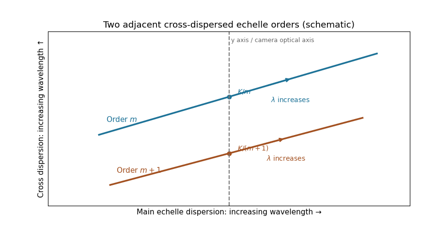


For fixed incidence, , so increasing wavelength goes to the right along each order. The cross-disperser also sends increasing wavelength upward in the chosen orientation; the traces therefore slope upward. At , , so the trace labeled lies above the trace labeled . Reflecting either plotting axis would reverse its arrow but leave the optical content unchanged. The cross-disperser separates orders that would overlap in the main dispersion direction.
Let be the direction of the optical camera optical axis. The grating equation on that axis isThe central wavelengths in adjacent diffraction orders are therefore and , with separation is the fixed order-times-wavelength product directed onto the optical camera axis, or the optical path difference between adjacent grooves in that direction. In a Littrow configuration, . This adjacent-central-wavelength spacing is a conventional free spectral range of an echelle grating; at high order it is approximately .
There is a qualification in the wording of the printed definition. The exact interval for which order lies closest to the axis is not, in general, identical to the spacing of two adjacent order centres. For a concrete counterexample take , , and a photodetector mapping . Equality of the distances from the axis for orders means , so their common boundary is . The other boundary with order is . Consequently the literal closest-order interval has widthfor and accessible non-grazing orders. This differs from the printed . For a nonzero , the exact boundary is determined by and need not even have the simple half-order form. The two definitions agree to leading order when is large. Thus the printed expression is correct as an adjacent-centre convention or a high-order coverage estimate, rather than an exact consequence of the literal nearest-axis definition. Gap-free coverage should be checked using the actual photodetector mapping and neighbouring order endpoints.
The optical pupil mapped onto the deformable mirror has actuator pitch approximately . A sinusoidal wavefront error must have at least two actuator intervals per period to avoid aliasing, by the Nyquist–Shannon sampling theorem. ThusIf the actuator centres include both endpoints of the optical pupil diameter, the literal pitch is and the corresponding expression is ; the paper uses the customary large- pitch convention. At the exact Nyquist boundary one quadrature can be poorly sampled, and real influence functions and actuator coupling reduce useful correction near the cutoff. The result is an ideal sampling bound, not a guarantee of arbitrary correction at its endpoint.
Write spatial frequency in cycles across the optical pupil as . The previous result gives a maximum axial spatial frequency . If one counts one representative per positive-quadrant integer lattice point inside an isotropic disk , the continuum area estimate isThis is the geometric counting convention producing the printed formula. Lattice boundaries, the zero-frequency piston and axis points give lower-order corrections, so the formula is not an exact integer count.
The mode definition in the PDF is , hence and . It does not itself specify a two-dimensional lattice, its orientation, its independent wave phase components or a circular rather than square spatial frequency cutoff. Full-cycle integer frequencies correspond only to the even values of in that definition. A general real wavefront error also needs both sine and cosine quadratures, and distinct oblique orientations cannot all be identified with a single positive quadrant: the Fourier transform of a real wavefront has conjugate coefficients at and , rather than identifying every independent sign change of a component.
For comparison, a circular spatial frequency disk has approximately signed full-cycle lattice points, or conjugate pairs; two real wave phase components per pair restore approximately real degrees of freedom. A square spatial frequency support gives a different count. The circular physical optical pupil similarly has only about illuminated actuators. The printed is a quadrant area estimate under an extra counting convention; it is not a uniquely determined count of all independently correctable wavefront modes from the stated one-dimensional mode condition.
The speckle contrast of a sinusoidal wavefront error gives a peak modal wave amplitude . If all residual modes have that wave amplitude, their coefficient norm is . Substituting the printed quadrant count gives the intended expressionThere is a normalization issue if this quantity is called physical spatial root mean square wavefront error. For , the actual pupil-averaged value isOn an orthogonal full-period basis, and cross terms vanish. Alternatively, independent uniform random wave phases give this result after wave phase averaging, even on a circular optical pupil. With the same and equal contrasts the physical RMS is thenA single full-period cosine already demonstrates the issue: its RMS is , not . On the actual circular optical pupil, any nonconstant unit-peak cosine also has mean square strictly less than one; averaging over its wave phase gives exactly . On a finite circular optical pupil, phase-dependent mode overlaps can additionally matter. If a constant piston is removed before computing RMS, replace the mode Gram matrix by its centred optical pupil covariance. The printed value can be recovered as a modal coefficient norm, or by counting orthogonal peak-amplitude quadratures in the physical RMS; neither convention is specified by the quoted mode definition. This is the distinction between modal amplitude norm versus wavefront RMS, not a correction silently made to the PDF. Unequal residual contrasts require , so one speckle's alone cannot determine the total RMS. The weak-aberration approximation also requires the total wave phase error to stay small, not merely each coefficient separately.
An optical pupil ripple of spatial period diffracts starlight into two sidebands displaced by along the ripple's spatial frequency vector. Substituting the axial Nyquist period gives the deformable-mirror control radiusThe square actuator lattice has component cutoffs , hence an ideal square corrected region with this half-width in each photodetector direction. Its diagonal reaches times the axial radius; an isotropic conservative restriction is the inscribed disk. Using as the scale of a spatial resolution element, the square is about elements on a side and in area; the disk has about elements. These are angular area counts, not the quadrant coefficient count in part (ii).
A circular illuminated optical pupil has fewer active actuator degrees of freedom than the complete square array, and influence functions alter the usable boundary. Moreover one real wave phase deformable mirror produces conjugately related corrections at opposite speckles: arbitrary complex-field correction of both independent wave amplitude and wave phase errors generally needs additional control, or a restricted half-plane. The square therefore describes ideal spatial-frequency access, rather than a guarantee that every intensity element inside it can be independently set to zero. The Fourier-domain square control region is derived in Bordé and Traub's speckle-nulling analysis.
Use the ideal detection convention of one collected electron per detected photon; otherwise replace photon totals by detected electron totals using the quantum efficiency. Let be the summed measurement on the star patch and the independent background-only patch. After additive offsets are removed, their means are and . Independent Poisson distribution counts have variance equal to their mean, and a single read of detector pixels contributes to each patch's variance. ThereforeThe two factors of two arise from the independently measured background and the second patch's read noise, not from doubling the stellar signal. The formula assumes equal background means, independent detector pixels and patch measurements, one read per patch, and negligible dark current or other noise. Several exposure reads or correlated detector pixels require their own variance and covariance terms.
With constant detected rates, , . Squaring the previous signal-to-noise ratio in photon counting givesFor , nonnegative background and target , choose the positive root:The other root is nonpositive. With no read noise, this reduces to ; in a read-dominated short exposure it approaches . If , no positive target stellar signal-to-noise is attainable. A zero target can be assigned zero exposure, with its limiting interpretation when all noise terms also vanish. Real quantum efficiency or multiple reads modifies the rates or read-variance term before solving the quadratic.
Let . After offset subtraction, each summed image has mean analogue-to-digital units per detector pixel. For a constant detector conversion gain and independent Poisson distribution detected counts, : summing independent frames adds both their means and variances. Here is the mean of the sum, not one frame.
Write , . At high counts, the delta method gives . Independence therefore givesThus the formula is a high-signal gain estimation from flat-field ratios, not an exact identity for a ratio of random variables. A Poisson distribution denominator can even be zero at low counts. The exposures must be linear and unsaturated, offsets removed, and read noise negligible. Being close to saturation increases the signal but does not establish linearity; clipping or charge-induced correlations biases a variance estimate. A large ensemble of suitable detector pixels supplies the measured standard deviation. In normal photodetector terminology is collected electrons per ADU, consistent with detected photons here only under the stated unit-yield convention; see the instrument gain definition.
A stable multiplicative sensitivity factor at detector pixel changes both means to . The noise-free ratio is still one, so flat-field correction is not required merely to remove that fixed pattern from the mean ratio. This is the principal advantage of using two matched flats rather than the variance of a single image.
However, the photon shot noise is not cancelled. At high counts the conditional ratio variance is . Pooling detector pixels gives , where brackets denote a spatial average. If the formula uses , it returnsThe inequality follows from the Jensen inequality for on positive signals. For small fractional response variation, the relative bias is approximately minus its squared coefficient of variation. A locally nearly uniform region or a fit using detector pixel-dependent variances avoids this bias from mixing the harmonic mean with the arithmetic mean. Stable response cancellation also presumes the conversion gain itself is uniform; gain variations, offset errors or changing sensitivity do not obey that simple cancellation. The fixed response pattern cancels in the ratio mean; unequal shot-noise levels can still bias a globally pooled gain estimate.
For independent reads in each sum, read noise contributes in squared ADU units. HenceUsing the shot-noise-only formula therefore givesThe condition for negligible contamination is , equivalently a large number of collected electrons per individual frame compared with . Summing more identical-level frames does not change that ratio because both and the read variance scale with . Measure read noise from paired bias images, or fit mean versus noise variance across several illumination levels: the shot-noise slope determines detector gain, while the read term gives an intercept. If is known, the corrected positive solution satisfies . Offset subtraction removes the mean bias but not the read variance. Correlated read errors need a different covariance calculation.
If spatial illumination is stable between the two sums, it acts just like the sensitivity factor: the mean ratio remains one but each detector pixel has a different shot-noise variance. A whole-image standard deviation is disproportionately influenced by faint detector pixels, so substituting a global arithmetic mean signal generally underestimates detector conversion gain. If the illumination pattern differs between the sums, their noise-free ratio is not constant; its structure adds apparent variance and causes a further systematic error.
Use locally uniform signal bins or subregions, remove offsets, mask defective or saturated detector pixels, and propagate the local shot and read variances. In the stable-pattern case a useful alternative to pooling raw ratios is the normalized differenceAt high signal and negligible read noise, treating the denominator at its mean gives , independent of the illumination. Thus a variance fit or can use a spatially varying flat without the arithmetic/harmonic mismatch. Measured noisy denominators cause higher-order corrections, so independent or smoothed signal estimates can be preferable. Fit and subtract a genuine changing illumination pattern before noise analysis, using sufficient smoothing not to fit away the random noise. Arbitrary flat-field normalization without propagating its noise does not by itself recover the original gain.
If temporal variation is spatially uniform, summing all frames in each group still gives independent Poisson distribution totals, but their means may now be with ratio . At high counts and negligible read noise, direct propagation givesAfter dividing the ratio image by its measured mean , the appropriate estimator isThe original formula is recovered only for . Uniform brightness drift does not automatically create a spatial pattern or extra ratio scatter beyond these changed noise levels; its leading problem is unequal group normalization. Interleave the groups in time or pair exposures of comparable flux, measure their separate means, and propagate shot and read noise when rescaling. If the spatial pattern or photodetector sensitivity also evolves, the ratio develops systematic structure that must be modeled or those frames rejected. A normalization inferred from finitely many detector pixels introduces a small shared correlation, which vanishes in the large-pixel limit and can be included in a precise uncertainty analysis.
Articles by others on the same topic
There are currently no matching articles.