An eigenvalue of a matrix is a scalar for which for some nonzero eigenvector . Its corresponding eigenspace is
Write . The displayed matrix is the outer product , soIts column space is contained in and is nonzero because . Hence is a rank-one matrix.
The vector is an eigenvector with eigenvalue , and every vector in the orthogonal complement has eigenvalue . ThusSince is a direct sum of these eigenspaces, has an eigenbasis and is therefore a diagonalizable.
The normalizer of in isIt is the stabilizer of the subgroup under the conjugation action of on its subgroups.
Take . Since is a normal subgroup, ; it has the same order as , so it is also a Sylow subgroup of . The conjugacy assertion in the Sylow theorems supplies such thatConsequently , and thereforeThus , while the reverse inclusion is immediate because both factors are subgroups of . Hence
A sequence of functions converges uniformly to when, for every , there is an such thatfor every . Equivalently, in the supremum norm.
Yes. Fix and . Uniform convergence gives such that for every . Since the continuous function is continuous at , there is a such that implies . The triangle inequality then givesThis proves the uniform limit theorem: is continuous.
No. For each , , whereas for every . The pointwise limit on is thereforeThis limit is not continuous at . Since every is continuous, the uniform limit theorem rules out uniform convergence. Directly, for , whose supremum over is for every .
No. DefineEach is a differentiable function on , whileThus converges uniformly to the absolute value function , which is not differentiable at . Uniform convergence alone therefore does not preserve differentiability.
The Cauchy integral formula says that if is holomorphic on a neighbourhood of the closed disc , then for ,In particular, at the centre,for every .
If , the assumed bound gives , so . Otherwise define . Then and . Applying the centre formula and taking real parts givesThe continuous nonnegative function has integral zero, so it vanishes around the circle. Equality together with forces . This holds for every , hence throughout the disc. This is the equality case underlying the maximum modulus principle.
Introduce the Cauchy approximate identityIt is an approximate identity converging to the Dirac delta function , and . For a smooth rapidly decaying test function , integration by parts givesBy the definition of the derivative of the Dirac delta, . Therefore the limit as a distribution is
For a wavefunction , the probability density and probability current areMultiply the Schrodinger equation by , multiply its complex conjugate by , and subtract. The real potential energy terms cancel, leavingwhich is the probability continuity equation .
For a stationary state, , so and is constant in space. A normalizable wavefunction has vanishing current at spatial infinity, forcing this constant to be zero. By contrast the nonnormalizable plane wavehas stationary density and nonzero currentwhen .
The momentum operator in the position representation is . Differentiating the given Gaussian wave packet givesThe probability density is an even function, so the term proportional to the odd function has integral zero. Normalization supplies , and hence
In vacuum the Maxwell equations areSubstitution of the complex plane electromagnetic wave amplitudes into these equations givesThus the electric field must be transverse to ; taking the positive-frequency branch gives .
For , , and , the real fields areThe electric vector rotates with constant magnitude, so this is circular polarization. Its Poynting vector isThe Poynting vector is the electromagnetic energy flux: its direction is the direction of propagation and its magnitude is the power crossing unit area.
Gaussian elimination without row exchanges gives the LU decompositionBecause has unit diagonal and is upper triangular,
Let be the number of returns to after time . Since is a recurrent state, the probability of another return after each visit is one. By the stated geometric distribution description, for every positive integer . Thus almost surely and .
On the other hand, writing each visit as an indicator random variable and applying the monotone convergence theorem to the partial sums givesThe left side is infinite, proving the recurrence criterion by return probabilities in the required direction:
By independence of the two simple random walks, linearity of expectation, and symmetry of their transition probabilities,The Chapman-Kolmogorov equation identifies the inner sum as , soA simple random walk on the integer line can return to only at an even time. Since it is recurrent at , part (a) givesTherefore .
For , define by . If , then in particularso . Thus is injective. Since a finite-dimensional vector space and its dual space have the same dimension, is also surjective and hence an isomorphism. This is the finite-dimensional real case of the Riesz representation theorem.
The adjoint operator of is the unique linear map satisfyingfor every and . In the stated orthonormal bases, if and denote coordinate columns, thenTherefore the matrix of is the matrix transpose .
For ,Hence . Taking orthogonal complements in the finite-dimensional space proves the image-kernel orthogonality for an adjoint
Put . For any ,This is minimized at exactly when , equivalently when . Thus the normal equation for a linear inverse problem is
A Smith normal form of an matrix over a principal ideal domain is a diagonal matrixwhere and . It is guaranteed to exist for every matrix over a principal ideal domain. The entries are determined up to multiplication by units; over they are conventionally chosen positive.
Present a finitely generated abelian group as the cokernel of an integer matrix . Changing by the invertible row and column operations used in its Smith normal form does not change the isomorphism type of the cokernel. Ifthenwhere factors with may be omitted. This is the Fundamental theorem of finitely generated abelian groups; the rank of an abelian group and invariant factors are unique.
There aresuch conjugacy classes. Every matrix in is an invertible matrix, so by the minimal polynomial of an invertible matrix its minimal polynomial must have nonzero constant term. Buthas constant term zero and cannot be the minimal polynomial of an invertible matrix.
Let be a Cauchy sequence in a compact metric space . By sequential compactness of a compact metric space, it has a convergent subsequence . Given , choose such that whenever , and then choose such that and . For every , the triangle inequality givesThus the whole sequence converges to . Every Cauchy sequence converges in , so is a complete metric space.
No. Give an infinite set the discrete metricThis space is bounded. Every Cauchy sequence is eventually constant, so it is complete. However, the open cover by the singleton balls has no finite subcover. Hence is not compact.
For any , the balls form an open cover of the compact metric space . Compactness supplies a finite subcoverThis is exactly total boundedness.
Let be any sequence in a complete, totally bounded metric space . Cover by finitely many balls of radius ; one contains infinitely many terms. From those terms choose an infinite subsequence lying in one ball of radius , and continue. The diagonal argument produces a subsequence whose tail from its th term onward lies in a ball of radius . Hencewhenever , so the subsequence is Cauchy. Completeness makes it converge in .
Every sequence in therefore has a convergent subsequence, so is sequentially compact. Sequential compactness is equivalent to compactness for metric spaces, and thus is compact. This proves that a complete totally bounded metric space is compact.
The space is not compact because it is not complete. For , define the continuous functionThese functions converge in the L1 norm to the step function , because is supported on an interval of length and bounded in absolute value by one. They are consequently Cauchy for the metric , since for sufficiently close pairs the outer minimum with does nothing.
If converged in this metric to some , it would also converge to in . Uniqueness of an limit would give almost everywhere. Continuity would then force on and on , which is impossible at . Thus this Cauchy sequence has no limit in , while every compact metric space is complete.
If , the subspace topology on isIf is an equivalence relation on and is the natural projection, the quotient topology declares open exactly when is open in . For topological spaces and , the product topology on has as a basis all sets with open in and open in .
A closed set is compact because it is closed in the compact space . Its image is compact by the fact that a continuous image of a compact space is compact, and every compact subset of the Hausdorff space is closed. Thus the continuous bijection is a closed map. Its inverse is consequently continuous, so is a homeomorphism. This is the compact-to-Hausdorff continuous bijection theorem.
Define a continuous map by the standard embedded torus of revolution parametrizationIts image lies in becauseThe periodicity of the trigonometric functions makes and , so is constant on every -equivalence class. The universal property of the quotient topology therefore gives a unique continuous map
Every point of has cylindrical radius between and , so its polar angle determines modulo one, while the pair on the unit circle determines modulo one. Hence is surjective, and two parameters have the same image exactly when they differ by the endpoint identifications defining ; thus it is injective.
The quotient is compact as the continuous image of the given compact space under the quotient map. The surface is Hausdorff because it has the subspace topology inherited from . The compact-to-Hausdorff continuous bijection theorem now shows that is a homeomorphism. Therefore
The Bromwich inversion formula givesFor , close the Bromwich contour in the left half-plane. The only enclosed singularity is the double pole at , whose residue isThe residue theorem therefore yields
Taking the Laplace transform in and using the initial condition , the radial heat equation in three dimensions becomesPut and . ThensoFiniteness at the centre forces .
The transformed boundary condition isSincesubstitution and cancellation of the two terms givesHenceand the required explicit transform is
Taking and using givesSet . The Taylor series of the denominator isConsequentlyThe singular part at is thereforeUsing long-time asymptotics from a Laplace transform and part (a), the centre temperature has late-time behaviour
The groupacts on the Poincare half-plane model byA direct calculation givesThereforeso every element of PSL2(R) is an isometry of the hyperbolic metric.
A Geodesic in the Poincare half-plane model is a vertical line or a semicircle orthogonal to the real axis. Given a hyperbolic line , choose a real Möbius transformation sending its two ideal endpoints to and . After multiplying its representing matrix by a scalar and, if necessary, changing its sign, it represents an element of and sends to the positive imaginary axis .
The chosen point then maps to for some . The dilation , represented byfixes and sends to . Thus every pointed line can be sent to , proving transitivity on pointed hyperbolic lines.
An orientation-preserving isometry fixing every point of fixes more than two points in the upper half-plane and hence, as a Möbius transformation, is the identity. The mapfixes pointwise and preserves the hyperbolic metric; it is the hyperbolic reflection in . Consequently the pointwise stabilizer is exactly
For any isometry , use part (a) to choose that agrees with on one pointed line and its tangent direction. Then fixes that line pointwise, so it is either the identity or its reflection. Hence the Isometry group of the Poincare half-plane consists ofandwith real coefficients, modulo multiplication of all four coefficients by a nonzero scalar.
Because the half-plane metric is a conformal rescaling of the Euclidean metric, its angles are Euclidean angles. For each , the hyperbolic lines meeting the imaginary axis at a fixed angle at are the Euclidean circleswhere denotes the vertical coordinate. These circles have centres on the real axis and are therefore hyperbolic lines; varying gives the required collection.
To construct a triangle, put one vertex at and a second at on , with . Draw from these vertices the lines making interior angles and with . Their Euclidean centres and radii areIf their other intersection has angle , the law of cosines in the Euclidean triangle formed by the two centres and that intersection givesEquivalently,The right side is greater than one exactly when . Since ranges continuously and strictly increasingly from to infinity for , such a exists. The three lines therefore bound a hyperbolic triangle with the prescribed angles.
Yes. By an element of , part (a) puts the side between the - and -vertices on and the first vertex at . A reflection if needed puts the triangle on the chosen side. The remaining freedom is the ratio of the heights of the second and first vertices, and the equation from part (c) determines it uniquely because is strictly increasing on . The two incident circles are then fixed, so their other intersection and the triangle are fixed. Thus triangles with the same three angles are isometric, which is Hyperbolic AAA congruence.
Write the admissible variation as , where at both ends. Differentiating the functional under the integral sign gives the first variationAfter integration by parts, with the boundary term vanishing,Thus the Euler-Lagrange equation isA second differentiation gives the second variation
The integrandis nonnegative, so . If , both continuous summands vanish everywhere. Hence , so is constant; the common boundary value forces . Conversely, has and , so . Therefore
This agrees with part (a): at , the first variation vanishes because , andThus the constant configuration is a stationary local minimum as well as the global minimum identified directly.
For , completing the square gives the Bogomolny boundConsequentlywith equality exactly when the Bogomolny equationholds everywhere. Separating variables, or differentiating the proposed form directly, gives all solutions with the required limits:These are the translated phi-four kinks.
Differentiating the first-order equation yieldswhich is precisely the Euler-Lagrange equation from part (a). Thus every configuration saturating the first-order bound is automatically a stationary solution of the second-order variational equation.
Let . Repeated integration by parts gives the formal adjoint rulesThereforeEquality of the coefficients of in and requiresso . This also makes the zeroth-order coefficients equal because . Hence, under boundary conditions that remove the boundary terms,This is the self-adjoint fourth-order scalar differential operator .
With and , the equation isMultiply by the real eigenfunction and integrate over . The clamped boundary conditions at both endpoints eliminate all boundary terms, soSince , the right side is a sum of nonnegative terms. It cannot vanish for a nonzero eigenfunction: if , the boundary conditions force . Thus
For and , the linear ordinary differential equation is , whose general solution isBy the stated parity reduction, an even eigenfunction has the form . The conditions have a nonzero solution exactly whenthat is,An odd eigenfunction has the form , and the corresponding determinant givesThus is an eigenvalue precisely under one of the two stated conditions.
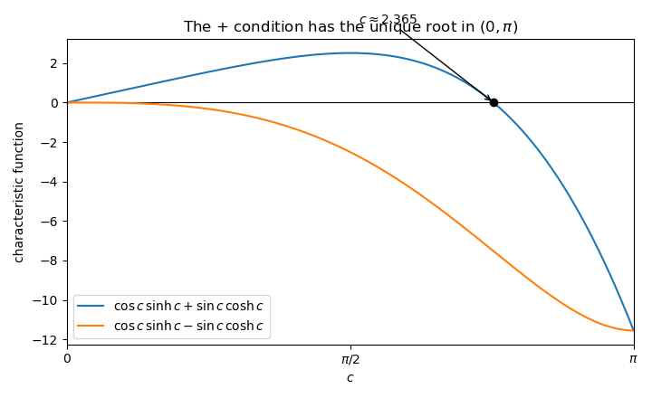
The fourth-order eigenvalue condition and its roots
. For the minus sign, division by away from gives . On , for , while on their signs differ, so there is no root. For the plus sign the equation isThere is no root in . On , the function increases strictly from to , so it has exactly one root by the intermediate value theorem. Numerically,Hence the combined condition has exactly one solution in .
The constant is the positive Coriolis parameter at northern latitude , is the gravitational acceleration, and is the undisturbed mean depth of the layer.
The linearized shallow water equations assume a homogeneous, incompressible, inviscid layer over a flat bed; a horizontal scale much larger than the depth, so the shallow-water approximation and hydrostatic approximation apply; depth-independent horizontal velocity; a free-surface displacement and sufficiently small velocity to neglect nonlinear products; and an f-plane on which is constant. The equations also omit viscosity, forcing, and bottom topography.
The vertical relative vorticity isDifferentiate the -momentum equation with respect to and the -momentum equation with respect to , then subtract. The mixed pressure derivatives cancel, givingThe mass-conservation equation says . Therefore the linearized shallow-water potential vorticitysatisfiesThus
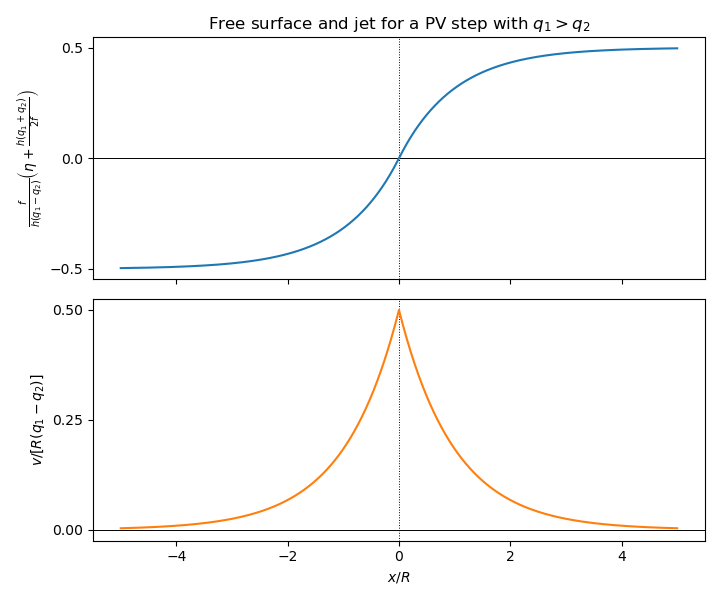
For a steady flow independent of , geostrophic balance givesHence , and the definition of becomesEquivalently,With the Rossby deformation radius , the bounded solution for the stated potential-vorticity step isContinuity of and at givesThereforeand
When , the surface height increases smoothly from to , while is a positive eastward jet with its maximum at the discontinuity and exponential decay on the Rossby-radius scale:
Articles were limited to the first 100 out of 117 total.
Articles by others on the same topic
There are currently no matching articles.