A basis of a vector space is a family of vectors that is both linearly independent and a spanning set of .
Write the given finite basis as . First, any other basis must also be finite. Each is a finite linear combination of elements of , so the union of the finitely many elements of occurring in these expressions is finite. Since spans every , it spans . If some existed, then would lie in the span of , contradicting the linear independence of . Hence ; write .
It remains to prove the elementary Steinitz exchange lemma directly. If independent vectors lie in the span of , express in terms of the . Some coefficient is nonzero, so the corresponding can be solved for in terms of and the other ; replacing it by preserves the span. Inductively, after replacing of the by , the expression for must have a nonzero coefficient on one of the unreplaced , since otherwise would be a linear combination of . That can again be replaced. There are only original vectors to replace, so .
Apply this argument first to the independent family and the spanning family to obtain , and then with the two bases interchanged to obtain . Therefore
The partial fraction decomposition isFor , expand both denominators by the geometric series:This is actually a Taylor series at zero, since the apparent puncture at zero contains no singularity.
For , the term still expands in nonnegative powers, while the quadratic term must be expanded in negative powers:Hence
For and , the Möbius transformationis an isometry of the disc, and every orientation-preserving disc isometry has this form. In particular, sends to zero and to a point of modulusRotations are also isometries, so it remains only to integrate the metric along a radial geodesic from to :Thus the Hyperbolic distance in the Poincare disc is
Introduce the orthogonal coordinatesThen the constraint and objective becomeThe Lagrange multiplier equations for a stationary point areIf , then and , givingIf , then . The first two equations and the constraint implyConverting back to gives the other four points. Therefore all stationary points arewith matching signs, together withThe middle pair has , the last pair has , and the first pair has .
Take down the plane and normally away from it, with the solid at and the free surface at . A steady unidirectional falling film flow has velocity . The streamwise Navier-Stokes equation reduces towhere is the kinematic viscosity. The lower no-slip boundary condition and upper stress-free boundary condition areIntegrating gives the velocity profileThe volume flux per unit width is
If the upper surface is replaced by a stationary solid plane, the second boundary condition becomes . The resulting plane-channel profile and flux areThe free surface exerts no tangential shear stress, whereas the stationary upper wall enforces no slip and exerts a retarding shear. This additional drag accounts for the reduced flux.
For distinct interpolation nodes , define the degree- divided difference byIt is the leading coefficient of the unique degree-at-most- interpolating polynomial through those data.
DefineThe partial polynomial agrees with at . Moreover, the explicit formula for the divided difference givesso . Induction shows that for every . By uniqueness of polynomial interpolation, this is the required Newton interpolation polynomial.
For the recursion, substitute the explicit formulas for and . For an interior index , the coefficient of in their difference isThe endpoint terms satisfy the same identity directly. Dividing by therefore gives
For observations , the log-likelihood of the normal distribution model isDifferentiating first with respect to gives . Substituting this value and differentiating with respect to gives the normal mean and variance maximum-likelihood estimators
An unbiased estimator of a parameter satisfies for every permissible value of . Since the sample mean is linear,so is unbiased.
Use the identityThe two expectations on the right are and , respectively. HenceThusThe unbiased sample variance instead divides the same sum of squares by .
Because is an interior minimizer of the differentiable function , it satisfies . Apply the Taylor theorem with Lagrange remainder to about . For some between and ,The lower bound on ensures that every step of the Newton method is defined. Divide by and useto obtain the exact error relationThe assumed derivative bounds now give the quadratic convergence bound for Newton's methodfor every .
The adjugate matrix is the transpose of the cofactor matrix, and it satisfiesPut and substitute the two given expansions into this identity:Comparing coefficients of powers of givesHere because the characteristic polynomial is monic.
Let . Expanding the determinant along row shows thatwhere is the corresponding cofactor. Since a diagonal entry of the adjugate matrix is that same cofactor, the multivariable chain rule along the diagonal yieldsTherefore
Taking the matrix trace of the adjugate expansion and using part (b) givesHence . Taking traces in gives, for ,For , the same formula follows by taking the trace of . Iterating the recursion from part (a) also givesConsequently the Faddeev–LeVerrier algorithm isStarting with , this recursively expresses every using only ; these are the Newton identities for the characteristic polynomial.
The group is a nontrivial finite p-group, so the nontrivial center of a finite p-group gives . If , then is already a nontrivial proper normal subgroup, so is not a simple group. If , then is abelian. By Cauchy's theorem for finite groups, it has a subgroup of order ; every subgroup of an abelian group is normal, and this subgroup is nontrivial and proper because . Thus in every case
Interchange the two primes if necessary so that . By the Sylow theorems, the number of Sylow -subgroups satisfiesIf , then is or . The first is impossible because . The second would implySince is prime, it cannot divide , so it must divide . But then forces , impossible because and are both odd. Therefore . The unique Sylow -subgroup is a nontrivial proper normal subgroup, and hence
A map is differentiable at when there is a linear map such thatThe linear map is the Frechet derivative of at .
The multivariable chain rule states that if is differentiable at and is differentiable at , thenIndeed, write and , where and . Since ,and the last two terms are . This proves the formula.
For matrix inversion near the identity matrix,The last term is because inversion is bounded near . Therefore the inversion map is differentiable at and
For every invertible matrix ,The maps and are linear. Differentiate this identity at and use the chain rule and part (a):Thus . Given an arbitrary increment , set to obtain the derivative of matrix inversionThis also proves differentiability at every .
For three sequences , if and agree through coordinate and and agree through coordinate , then and agree through coordinate . Henceand thereforeThus is a metric; in fact, the stronger first inequality makes it an ultrametric.
Let be a Cauchy sequence in , where . For each positive integer , choose such thatThis inequality says that the first coordinates of and agree. Consequently each coordinate is eventually constant. Let be its eventual value and put .
If were a continuous path, then would be a continuous map from the connected interval to a discrete space, so it would be constant. This holds for every , and therefore itself must be constant. Since contains distinct points, no path joins every pair. Henceindeed, every path component is a singleton.
Jordan lemma states that if and is analytic in the upper half-plane outside a fixed circle, withthen on the upper semicircle ,Indeed, . Using symmetry and on gives
The residue of at an isolated singularity is the coefficient of in its Laurent series, equivalentlyIf , the Taylor expansion of the analytic function shows that
For the real integral, apply contour integration in the upper half-plane toJordan's lemma removes the semicircular arc. The only enclosed singularity is the double pole at , whose residue isThe residue theorem therefore givesIts real part vanishes because is an odd function, while its imaginary part is the requested integral. Hence
Since , the function on the left of the defining expansion is . Thereforewhich is the two-dimensional Helmholtz equation.
In polar coordinates,Substitute the defining Fourier cosine series and equate the coefficient of each . Its angular second derivative contributes , so every Bessel function satisfiesor equivalently the Bessel differential equation
The Time-dependent Schrodinger equation for the one-dimensional Quantum harmonic oscillator isA stationary state has , so cancellation of the common time factor gives
If is monic of degree , the coefficient of in this equation is . It must vanish, soWriting gives the recurrenceThe coefficient of first gives , and the recurrence preserves parity. If is even, every odd coefficient vanishes, so is an even function. The Gaussian factor is also even; therefore the stationary state has even parity.
Use and Gauss's law . The divergence theorem and the decay at infinity giveMultiplying by proves that the two expressions for the electrostatic energy agree.
The uniform volume charge density in the thick shell isSpherical symmetry and the integral form of Gauss's law giveThus is zero inside, rises continuously through the charged region, reaches at , and then decays as . Taking and integrating givesThe electric potential is continuous, constant inside, decreases smoothly across the charge, and continues as outside.
As , the charge becomes a surface shell. ThenThe potential remains continuous, but the normal electric field jumps by across the surface charge density.
The field-energy expression givesThe charge-potential expression gives the same result directly because the entire charge lies where the potential equals :This is the electrostatic energy of a uniformly charged spherical shell.
Since is proportional to ,to first order. This is the work required to bring the additional charge from infinity to the potential created by the charge already present.
For an incompressible flow, . If the flow is also irrotational, then locally for a velocity potential, and therefore
The boundary conditions areThe fluid region is not simply connected, so a potential may change by the constant after one circuit while its gradient remains single-valued. Superposing uniform flow, the cylinder doublet, and the circulation gives the potential flow around a circular cylinder with circulationIts velocity components are
On , and, with ,The Bernoulli equation gives . The pressure force per unit length on the cylinder isThe component vanishes by symmetry, while givesin agreement with the Kutta–Joukowski theorem.
A stagnation point satisfies . On the cylinder this means . Thus gives two surface stagnation points, gives one coincident surface point, and gives none on the surface. Away from the cylinder, requires . Solving then gives one physical exterior root when :At this root lies on and agrees with the single surface point.
Insert the exact solution into the linear multistep method and expand about . Its defect isThe coefficient of isfor , while the constant coefficient is . The method has order at least exactly when these coefficients vanish for .
On the other hand,The coefficient of in this expression is precisely the preceding order-condition coefficient. Therefore all coefficients through degree vanish exactly whenwhich proves the equivalence.
For this Adams–Moulton method, the characteristic polynomials of a linear multistep method areExpansion at zero givesPart (a) therefore shows that the method has order exactly three.
It is consistent because its order is at least one. The roots of are and ; both lie in the closed unit disk, and the only unit-modulus root is simple. Thus the method is zero-stable. By the Dahlquist equivalence theorem, consistency and zero stability imply convergence. Hence the method is
The Neyman-Pearson lemma says that for simple hypotheses with densities , a size- test that rejects where and accepts where , with possible randomization on equality to attain size , is most powerful among all tests of size at most . To prove it, let be this test and any competing test. Pointwise,After integration,which proves maximal power.
For the exponential sample, with ,Since , this ratio is increasing in . The likelihood-ratio test therefore rejects for large :where is the distribution function of the rate-parameterized Gamma distribution .
The power function of a test is the probability of rejection as a function of the true parameter. Since ,At the null value, .
A level- test is uniformly most powerful for a composite alternative when its power is at least that of every other level- test at every parameter value in that alternative.
For every fixed , the likelihood ratio is increasing in the same statistic , and the size- threshold is always the null quantile , independent of . The Neyman-Pearson lemma therefore makes the test from part (a) most powerful against every individual . Consequently it is
By the definition of conditional probability and stationarity,This is the transition matrix of the time-reversed Markov chain.
Conditional on , the random variable is the first return time . The Kac's lemma mean-recurrence formula for a finite irreducible Markov chain givesAveraging over therefore yields
Let the common initial state be and the robber's final state be . Part (a) gives their joint distribution asLet be the cop's hitting time of when starting from . For a chain started from , condition on its first step to obtainHence the expected catch time, averaged over the displayed joint law, isUsing Kac's lemma once more givesThe convention correctly counts an immediate catch when the robber's reverse step leaves it at the common starting state.
Let . Choose a basis of the intersection of vector subspaces, extend it to a basis of , and independently extend it to a basis of . The combined listspans the sum of vector subspaces . It is also linearly independent: a vanishing linear combination says that a combination of the belongs to , and its expression in the chosen basis of forces all its coefficients to vanish; the coefficients of the then vanish in the same way. This proves the dimension formula for a sum of subspaces
Parametrize the two linear subspaces asPutting a vector of in first forces its fourth coordinate to vanish; the remaining defining equation is then automatic. Thusand the dimension formula gives .
The linear functionalvanishes on each displayed generator of and . Its kernel is three-dimensional because , so the inclusion between two three-dimensional subspaces is equality.
Let the torsion submodule of the module over a ring beThis is a submodule. Indeed, if and with , then because the scalar ring is an integral domain, and ; scalar multiples and additive inverses are handled similarly.
Take the quotient module and let be the quotient R-module homomorphism. It is torsion-free: if and , then , so for some . Since , this puts in and therefore .
Now let be torsion-free and let be an -module homomorphism. If and for , then , so torsion-freeness gives . Hence , and the universal property of a quotient module gives a unique homomorphismwith . Thus is the maximal torsion-free quotient of .
For , all component functions are continuously differentiable and the Jacobian matrix isAt a point , the first component cannot be differentiable: along the first coordinate axis its difference quotient contains , which is unbounded as . Therefore is continuously differentiable exactly at the points with .
At a point with , the determinant of the derivative isThe inverse function theorem therefore supplies neighbourhoods on which has a continuously differentiable, hence differentiable, inverse. Concretely, if , the local inverse is the restriction ofwhich is continuously differentiable near the image whenever .
Suppose for contradiction that the continuous image of a connected space is disconnected. Then there are disjoint nonempty sets , open in the subspace topology on , with . By continuity, and are disjoint open subsets of ; by surjectivity both are nonempty, and their union is . This is a separation of a topological space of , contradicting that is a connected space. Hence is connected.
First recall from the least-upper-bound property that every real interval is connected. For completeness, if were a separation with , let be the supremum of the points for which remains in . Relative openness rules out both and : in the first case one can move slightly to the right while staying in , and in the second one finds points of slightly to the left of , contrary to the definition of . Thus no separation exists.
Part (a) now makes a connected subset of the real line. Such a set is an interval: if it contained but omitted , its intersections with and would separate it. Since contains and , it consequently contains every number between them. Therefore for each such there is an with . This derives the intermediate value theorem from connectedness.
For an axisymmetric separated solution of the Laplace equation whose angular factor is the Legendre polynomial , the radial ordinary differential equation has the two powers and . Thusfor constants .
Write . Since , only the spherical harmonics of degrees zero and two occur. The degree-zero radial coefficient satisfying its two Dirichlet boundary conditions is . For degree two, write ; thenso and . By linearity and uniqueness of this boundary value problem,Direct substitution at verifies both boundary values.
The free-space Green function of the Laplacian for the Poisson equation gives the electric potentialFor , its electric multipole expansion begins withDefine the total electric charge and electric dipole moment byThen
The analogous solution for the magnetic vector potential isIts apparent coefficient is . For each component, the supplied identity and the divergence-free vector field condition giveThe divergence theorem turns this into a surface integral outside the compact support of the current density, where . Hence , so the term vanishes.
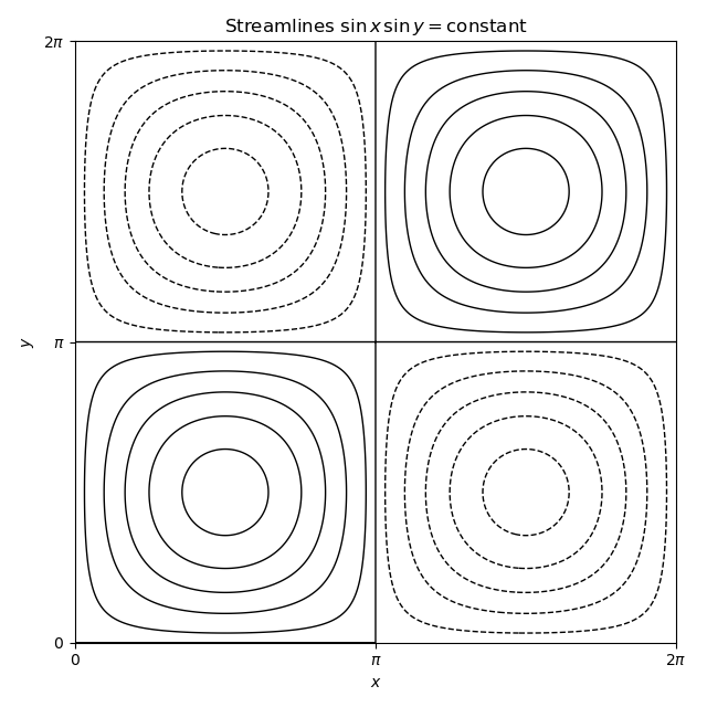
The velocity field is incompressible becauseWith the convention and , a stream function isThe vorticity is vertical:For a steady inviscid incompressible flow, the vorticity equation is . Here the right side is zero because the flow is independent of , while the left side is because velocity is tangent to the level sets of . Thus the equation is satisfied.
The streamlines are the level curves . The lines and , together with the boundary, are separatrices; each of the four cells contains closed nested curves around a centre at , , , or .
Let be the number of heads. The likelihood function for the Bernoulli distribution sample is proportional to . A uniform distribution prior on is the distribution, so Beta-binomial conjugacy gives the posterior distribution
Articles were limited to the first 100 out of 373 total.
Articles by others on the same topic
There are currently no matching articles.