Past exam of the mathematics course of the year 1 of the natural sciences course of the University of Cambridge / 2020 / Paper 1

Write the remaining quadratic polynomial as $x^2+bx+c$. Comparing coefficients in $(x-2)(x^2+bx+c)$ with the given cubic polynomial gives $b-2=-1$ and $-2c=-2$, hence $b=c=1$. The coefficient of $x$ is then $c-2b=-1$, as required. Thus

The Pythagorean trigonometric identity makes the second factor $1+{\cos }^2\theta$, which is strictly positive. It is therefore enough to solve $\sin \theta -\cos \theta \le 0$. The sine addition formula givesThe shifted angle lies between $\pi /4$ and $5\pi /4$. On this interval the sine is nonpositive precisely from $\pi$ onwards. Restoring the original angle and retaining its strict upper bound gives

Apply the product rule to $x\sin (1/x)$ and the chain rule to the sine. Since $d(1/x)/dx=-1/x^2$, the derivative is

Set $X=x^2$ and $Y=y^2$ in the two conic sections. A real intersection requires $X,Y\ge 0$. Solving the resulting linear equations givesFor $a>0$ the denominator and $X$ are positive, so intersections exist exactly when $a\ge 1$. At $a=1$ they are $(\pm 1,0)$; for $a>1$ both choices of sign for each square root give intersections. Consequently

The double-angle formula for the tangent function gives $1=2t/(1-t^2)$. Here $0<t<1$, because $0<\pi /8<\pi /4$, so the denominator is nonzero. Rearranging yields the quadratic equation

The quadratic formula gives $t=-1\pm \sqrt{2}$. The tangent function is positive in the first quadrant, so the positive polynomial root is selected:

Use integration by substitution with $u=3-2x$, so $dx=-du/2$ and $x=(3-u)/2$. The indefinite integral becomesThus, with an arbitrary constant of integration,This real antiderivative applies for $x<3/2$ and extends continuously to the stated endpoint. Its left derivative there agrees with the limiting integrand, zero.

The two directed segments have vectors $\mathbf{u}=(1,0,-1)$ and $\mathbf{v}=(0,1,1)$. Their dot product is $-1$ and both norms equal $\sqrt{2}$. HenceThe common starting point fixes the obtuse angle between these segments.

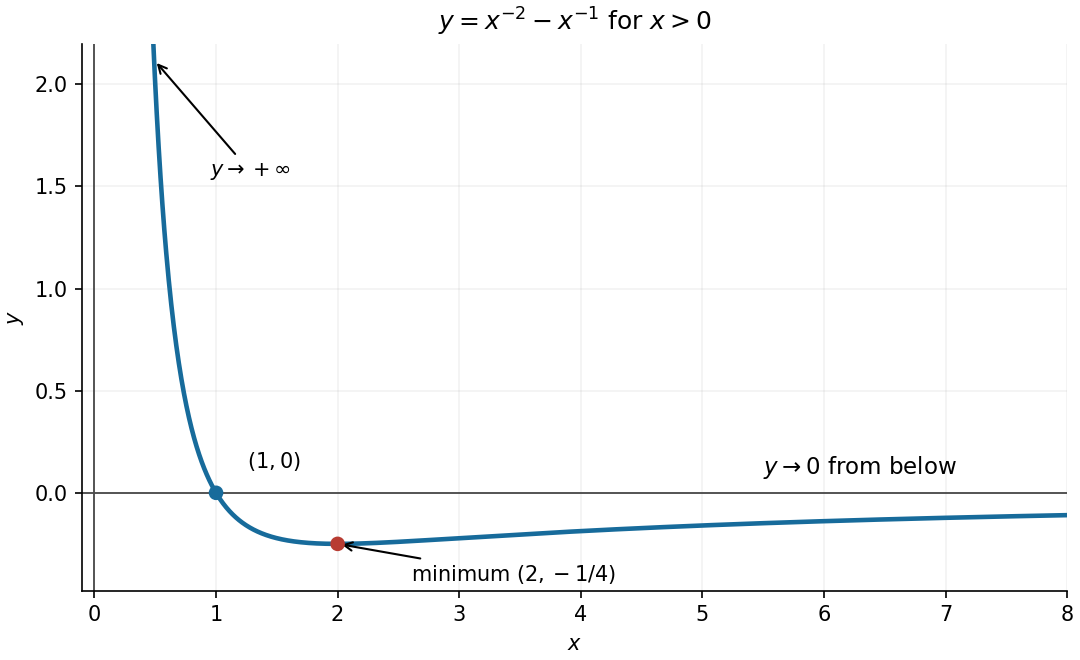
Differentiate the two powers to locate the stationary point:For $x>0$, this is negative before $2$ and positive afterwards, so the global minimum isThe curve crosses the horizontal axis at $x=1$. Its limits are $+\infty$ as $x\to 0^{+}$ and $0$ from below as $x\to \infty$, giving the vertical asymptote $x=0$ and horizontal asymptote $y=0$. These features determine the required sketch.

The first term is $ar$, so the finite geometric series is $S=a(r+r^2+\cdots +r^{100})$. Subtracting $rS$ cancels the interior terms and gives $(1-r)S=ar(1-r^{100})$. ThereforeThe rational expression holds for every real $a$ and every real $r\ne 1$, including $r=0$; the same algebra works for complex numbers. No restriction $|r|<1$ is needed for a finite geometric series. The exceptional case follows by adding one hundred equal terms, or by taking the limit as $r\to 1$.

For this polynomial, $f^{\prime }(x)=2x$, so the specified Newton root-finding iteration simplifies toStarting at one gives $x_1=(1+2)/2=3/2$, followed by $x_2=(3/2+4/3)/2=17/12$. Consequently

Multiply numerator and denominator by the complex conjugate $2+i$:Thus the real part and imaginary part are

Powers of the imaginary unit repeat in blocks $i,-1,-i,1$, each with sum zero. The first $44$ terms comprise eleven complete blocks; the last is $i^{45}=i$. Applying Euler's formula to the resulting complex exponential gives $e^i=\cos 1+i\sin 1$. HenceThe angles here are in radians.

The exponential definitions of hyperbolic sine and hyperbolic cosine, together with Euler's formula, give $\sinh (iu)=i\sin u$ and $\cosh (iu)=\cos u$. The argument of the complex logarithm therefore reduces to $i\sin (\pi /2)+\cos (9\pi /2)=i$.

Using the principal logarithm, $\log i=i\pi /2$, soIf no branch of the complex logarithm is selected, its complete set of values is $i(\pi /2+2\pi k)$, $k\in \mathbb{Z}$. The real part remains zero, while the imaginary part is $\pi /2+2\pi k$. The original paper does not explicitly state a branch convention.

The literal expression in the original PDF is undefined. Indeed, hyperbolic tangent satisfies $\tanh w=\sinh w/\cosh w$, andAlready the $n=2$ summand contains $\tanh (i\pi /2)$, a pole. The shifted term has the same issue when $n\equiv 3(\mathrm{mod}4)$. Thus this is not a finite sum of defined complex numbers, and it has no literal real or imaginary part. Cancelling two undefined terms is not ordinary arithmetic.

There is nevertheless a natural interpretation by meromorphic telescoping cancellation. Insert the same small positive real shift $\epsilon$ into every hyperbolic tangent argument. Each term is then finite, and the telescoping sum isSince hyperbolic tangent has period $i\pi$, its first argument can be reduced to $\epsilon +i\pi /4$. Taking the limit givesThis is a common-shift continuation of the sum, plausibly the intended telescoping answer. It requires that additional convention; it is not the value of the expression as printed.

Write $z=x+iy$. Then $|z^{\ast }+2i|=\sqrt{x^2+(y-2{)}^2}$ and $|z|=\sqrt{x^2+y^2}$, so the condition fixes the sum of distances from $(0,2)$ and $(0,0)$. It is an ellipse with centre $(0,1)$, vertical semimajor axis $A=2$, and focal distance $c=1$. Its horizontal semiminor axis obeys $B^2=A^2-c^2=3$. Thus the locus isThe vertices are $(0,-1)$ and $(0,3)$; the horizontal extremities are $(\pm \sqrt{3},1)$. The complex conjugation places the second focus above the origin.

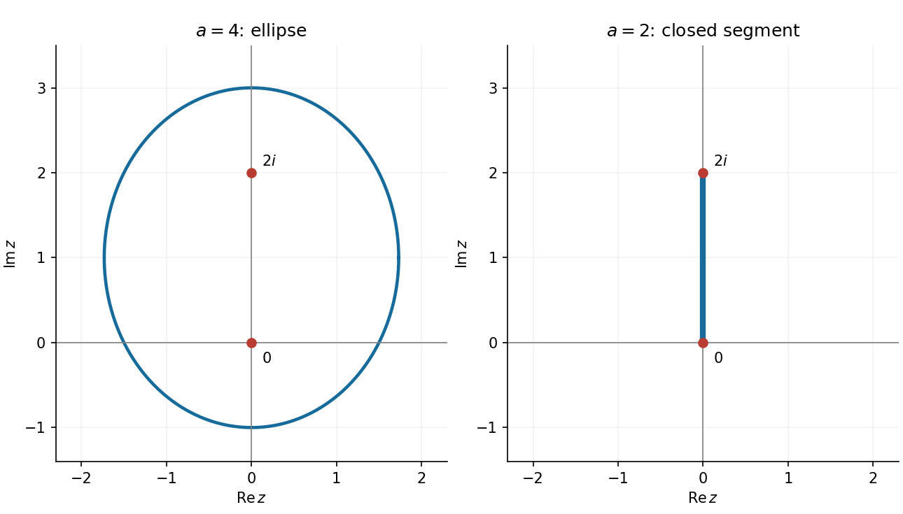
The triangle inequality bounds the distance sum below by the separation of the two foci, which is two. Equality holds exactly for points on the closed segment joining them. Hence the locus isBoth endpoints are included. It is the segment on the positive imaginary axis shown in the right-hand panel above.

For polar coordinates, $x=r\cos \theta$ and $y=r\sin \theta$. The Jacobian determinant is $r$, so the area element isThis accounts for the increasing length of an angular strip as its distance from the origin increases.

Let $I$ be the positive Gaussian integral. Its improper integral converges because $e^{-x^2}\le e^{-|x|}$ for $|x|\ge 1$. Multiplying two copies and using the polar coordinates area element givesNonnegativity justifies the product double integral and the change of integration order. Since $I>0$,

The cardioid has a nonnegative radial boundary, so each ray from the origin contributes $0\le r\le a(1+\cos \theta )$. Integrating the polar coordinates area element yieldsThe three angular integrals are $2\pi$, zero and $\pi$, respectively, using the double-angle formula for the last. Thus

The volume element is the absolute Jacobian determinant times the coordinate differentials. In the Cartesian coordinate system, cylindrical coordinates $(r,\theta ,z)$ and spherical coordinates $(\rho ,\vartheta ,\phi )$, respectively,Here $\rho$ is distance from the origin, $\vartheta$ is the polar angle from the positive $z$ axis, and $\phi$ is the azimuthal angle. The spherical coordinates convention fixes which angle enters the sine factor.

At height $z>0$, the elliptic paraboloid has a circular cross-section $0\le r\le \sqrt{z}$, of area $\pi z$. The cylindrical coordinates volume element therefore reduces the volume integral toFor the specified $f$, the derivative is $e^{-z}(z^{-1/2}+\frac{1}{2}{z}^{-3/2})$. Thus $z{f}^{\prime }(z)$ is integrable at zero and decays exponentially at infinity. Apply integration by parts first on a truncated interval and then take the endpoint limits:Both boundary terms vanish because $zf(z)=-\sqrt{z}{e}^{-z}$. With $z=u^2$, integration by substitution gives the Gaussian integral:The integrand is singular at the apex but the resulting improper integral is convergent.

In spherical coordinates, the cone condition forces $z\ge 0$ and becomes $0\le \vartheta \le \alpha$. The unit ball gives $0\le \rho \le 1$. HenceFor an independent calculation in cylindrical coordinates, the lower boundary is $z=r\cot \alpha$ and the upper boundary is $z=\sqrt{1-r^2}$. They meet at $r=\sin \alpha$, since $r^2{\cot }^2\alpha =1-r^2$. ThusThe equality uses ${\sin }^3\alpha \cot \alpha ={\sin }^2\alpha \cos \alpha$. The positive cosine on the stated range removes any square-root sign ambiguity.

For a first-order linear ordinary differential equation $y^{\prime }+p(x)y=q(x)$, an integrating factor is $\exp (\int p(x)dx)$. Here $p(x)=\cot x$, soThe sine is positive on the specified interval, so this integrating factor never vanishes there. Any nonzero constant multiple is equally suitable.

Multiplication by the integrating factor and the product rule turn the left side into a single derivative:Using integration by substitution $u=\cos x$ gives $y\sin x=-{\cos }^{3}x/3+C$. Therefore the general solution isThere is one arbitrary constant of integration, as expected for a first-order ordinary differential equation.

Insert the exponential function trial $y=e^{rx}$ into the homogeneous linear differential equation. Its characteristic equation is $r^2+\sqrt{3}r+3=0$, with polynomial rootsTaking real combinations of the two complex exponential solutions produces the general solution

Use the method of undetermined coefficients with a particular solution $K{e}^{-\sqrt{3}x}$. The differential operator multiplies this exponential function by $3-3+3=3$. Matching the forcing coefficient gives $3K=1$, hence

A linear polynomial trial $y=ux+v$ has $y^{\prime }=u$ and $y^{\prime \prime }=0$. Substituting gives $3ux+(\sqrt{3}u+3v)=x$, so $u=1/3$ and $v=-\sqrt{3}/9=-1/(3\sqrt{3})$. Thus a particular solution is

The superposition principle gives the general solution as $y_c+2y_{p,2}+y_{p,1}$:The first boundary condition gives $A=2/(3\sqrt{3})-1/3$. At $x=\pi$, the cosine vanishes and the sine equals $-1$. Comparing with the second boundary condition then givesThe unique solution satisfying both boundary conditions is thereforeUniqueness follows because a homogeneous solution zero at both endpoints would have $A=0$ from the first and $B=0$ from the second.

Put $s=x^2+y^2$. The gradient components areA stationary point requires both components to vanish. If $x\ne 0$, then $s=1$; the second component subsequently forces $y=0$, giving $(\pm 1,0)$. If $x=0$, either $y=0$ or, writing $u=y^2$,Only $u=1/2$ is nonnegative. Thus there are five stationary points, with valuesThe cases $x=0$ and $s=1$ exhaust the first partial derivative equation, so no other stationary points have been lost by division.

The Hessian matrix has entriesAt each stationary point the mixed entry vanishes, so the signs of the diagonal entries directly classify the local quadratic change:In particular the two local minima are also global minima: the squared term is nonnegative and $\ln (3+y^2)\ge \ln 3$, with equality in both bounds exactly at $(\pm 1,0)$. The local maximum at the origin is not a global maximum, since $f$ grows without bound as $x^2+y^2\to \infty$. The opposite diagonal signs at the other two points establish their saddle point character.

The contour plot is symmetric under either $x\mapsto -x$ or $y\mapsto -y$, because $f$ depends only on their squares. Denote the three critical heights by $m=\frac{7}{2}\ln 3$, $h=\frac{1}{4}+\frac{7}{2}\ln (7/2)$ and $M=1+\frac{7}{2}\ln 3$, where $m<h<M$.

For $m<c<h$, the level set $f=c$ consists of separate closed curves around the two minima. At $c=h$ the branches meet at the two saddle points. For $h<c<M$, there is an inner closed curve surrounding the local maximum and an outer closed curve surrounding all five stationary points. At $c=M$ the inner curve shrinks to the origin; for $c>M$ only the outer closed curve remains. At each saddle point the critical level set crosses in the two directions determined byThe figure plots representative level sets, including the critical saddle height; its second panel adds the gradient directions requested below.

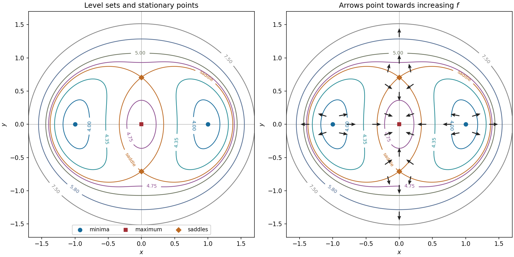
The gradient is orthogonal to each regular level set and points towards increasing $f$. Near either minimum, the linear approximation is $(8\delta x,\frac{7}{3}\delta y)$, so arrows point away from the point. Near the maximum at the origin it is $(-4\delta x,-\frac{5}{3}\delta y)$, so arrows point inwards. Near either saddle point it is $(-2\delta x,\frac{24}{7}\delta y)$: arrows point towards the vertical axis horizontally and away from the saddle vertically.

On the horizontal axis the gradient is $(4x(x^2-1),0)$. Its arrows point left on $x<-1$, right on $-1<x<0$, left on $0<x<1$, and right on $x>1$. On the vertical axis it isConsequently its arrows point down on $y<-1/\sqrt{2}$, up on $-1/\sqrt{2}<y<0$, down on $0<y<1/\sqrt{2}$, and up on $y>1/\sqrt{2}$. These directions, and representative arrows near each stationary point, appear in the right-hand panel. The gradient itself is zero at all five stationary points.

The finite form of Taylor's theorem with the first $n$ terms iswhere $\xi$ lies strictly between $a$ and $x$ for $x\ne a$. A sufficient hypothesis is that $f$ has continuous derivatives through order $n-1$ on the interval joining the endpoints and an $n$th derivative in its interior. The displayed polynomial has degree at most $n-1$; its Taylor remainder uses the $n$th derivative, not the $(n+1)$st. At $x=a$ the remainder is zero. This is a finite Taylor polynomial identity and does not require an infinite Taylor series to converge.

For $f(x)=x^{1/5}$, the first two derivatives are $f^{\prime }(x)=x^{-4/5}/5$ and $f^{\prime \prime }(x)=-4x^{-9/5}/25$. Since $32=2^5$,The first three terms of the Taylor expansion, with $x-32=1$, therefore giveFor a check on accuracy, $f^{(3)}(x)=36x^{-14/5}/125$ is positive and decreasing on $[32,33]$. The Taylor remainder is consequently positive and less than $f^{(3)}(32)/6=3/1024000<3\times 10^{-6}$. The approximation is a slight underestimate.

Divide numerator and denominator by $x$ before taking their Maclaurin series:For the reciprocal denominator, the geometric series gives $1-x^2/6+7x^4/360+O(x^6)$. Multiplying gives the Taylor expansionStrictly, the original quotient has a removable singularity at zero; this is the Taylor series of its continuous, analytic extension with value one there. The absence of odd powers also follows because the ratio of these two odd functions is even.

The definition of hyperbolic sine simplifies the composition exactly for $x>0$:Set $h=x-1$. The geometric series $1/(1+h)=1-h+h^2-h^3+h^4+O(h^5)$, valid for $|h|<1$, then gives

Random sampling without replacement assigns each of the ten distinguishable pieces to each lunch with the same probability. Five pieces of each type therefore giveOne can check the second probability by conditioning on the first lunch:The identical marginal probabilities do not imply independence of the draws.

Condition on an apple occupying position two in a uniformly random ordering. The nine other positions then contain four apples and five bananas, each equally likely to occupy position three. The conditional probability is thereforeThis uses exchangeability of the unconditioned positions; there is no need to assume the first lunch contained a particular fruit.

Each position has apple probability $1/2$. Applying Bayes' theorem to the preceding conditional probability givesThis also agrees with exchangeability of the second and third positions.

By the inclusion-exclusion principle for probabilities,After an initial banana, five of the nine remaining pieces are apples, so the intersection probability is $(1/2)(5/9)=5/18$. ConsequentlyAs a check, the complementary event is an apple followed by a banana, which also has probability $5/18$.

Let $I_j$ be the indicator random variable of an apple in lunch $j$. The number remaining is $R=5-I_1-I_2-I_3$. Each expected value $E[I_j]=P(A_j)=1/2$. The linearity of expectation therefore givesAlthough the indicator random variables are dependent under sampling without replacement, the linearity of expectation needs no independence assumption.

Let $N$ count rotten pieces. Each item supplies an independent Bernoulli trial with success probability $p$, so $N$ has a binomial distribution with parameters $10,p$. There are $\left(\genfrac{}{}{0ex}{}{10}{n}\right)$ choices of the rotten items, and each such choice has probability $p^n(1-p{)}^{10-n}$. HenceFor $p=0$ or $p=1$, interpret this as the corresponding distribution concentrated at zero or ten; no ambiguous $0^0$ evaluation is needed.