Past exam of the mathematics course of the year 2 of the natural sciences course of the University of Cambridge / 2020

Write the position vector as $\mathbf{r}(\rho ,\varphi ,z)=(\rho \cos \varphi ,\rho \sin \varphi ,z)$. Its coordinate tangent vectors areTheir pairwise dot products vanish. Their lengths, the scale factors of orthogonal coordinates, areThus the cylindrical coordinate system is orthogonal wherever it is a nonsingular coordinate chart. At $\rho =0$, the angular tangent vector vanishes and the azimuth is undefined; this is the usual coordinate singularity on the axis, not a failure of the Euclidean geometry.

Dividing the coordinate tangents by their scale factors of orthogonal coordinates gives an orthonormal basisEvaluate the Cartesian cross products componentwise:ConsequentlyThe ordered cylindrical basis is right-handed: its scalar triple product ${\mathbf{e}}_{\rho }\cdot ({\mathbf{e}}_{\varphi }\times {\mathbf{e}}_z)$ equals $+1$.

Differentiate the position vector, using the angular factor from the scale factors of orthogonal coordinates:The basis is an orthonormal basis, so all cross terms in its squared length vanish. The Euclidean line element is thereforeIn particular, an angular change $d\varphi$ at fixed radius traverses a physical distance $\rho |d\varphi |$.

For a finite separation use the Cartesian distance, rather than substituting finite coordinate differences into the local line element. Expanding the two horizontal components givesThe vertical contribution is $(z-z^{\prime }{)}^2$, independently. ThusandEquivalently, the horizontal contribution is $(\rho -{\rho }^{\prime }{)}^2+4\rho {\rho }^{\prime }{\sin }^2[(\varphi -{\varphi }^{\prime })/2]$, which also makes its nonnegativity explicit.

The radial unit vector in the spherical coordinate system isThe coordinate tangent in the polar direction has length $r$, so its corresponding unit vector isDifferentiating ${\mathbf{e}}_r$ at fixed $\varphi$ therefore givesThe factor is not $r$: the corresponding scale factors of orthogonal coordinates occur in the derivative of the position vector, whereas the question differentiates its unit direction. The formula is understood away from the coordinate singularities where a complete spherical basis is not uniquely specified.

Differentiate the power series term by term inside its radius of convergence, and reindex the second derivative so that every coefficient multiplies $x^m$. The differential equation becomesThe uniqueness of power-series coefficients givesThe even coefficients depend only on $a_0$ and the odd coefficients only on $a_1$. These are the two local solution branches of the Legendre differential equation around its ordinary point $x=0$.

For an integer $n\ge 0$, choose the series whose integer parity agrees with $n$ and set the other initial coefficient to zero. At $m=n$, the numerator in the recurrence vanishes, so $a_{n+2}=0$ and every later coefficient in that integer parity vanishes. With a nonzero coefficient of $x^n$, this gives a polynomial of degree exactly $n$. Normalize it by $P_n(1)=1$.

For $n=0$, the even branch is constant; for $n=1$, the odd branch is proportional to $x$. For $n=2$, the recurrence gives $a_2=-3a_0$, so normalization fixes $a_0=-1/2$. HenceThe opposite-parity branch generally does not terminate; polynomial termination does not mean that both independent solutions become polynomials.

Substitute $U=R(r)F(\theta )$ into the axisymmetric Laplace equation and multiply by $r^2/(RF)$. The radial and angular terms must be separate constants:ThusWith $x=\cos \theta$, the angular equation becomesRequiring boundedness on the entire polar interval, and using the supplied characterization of bounded Legendre polynomial solutions, gives $\lambda =n(n+1)$ and $F\propto P_n(\cos \theta )$ for $n=0,1,2,\dots$. Trying $R=r^s$ gives $s(s+1)=n(n+1)$, hence $s=n$ or $s=-n-1$.

The globally angular-regular separated modes and their superposition are thereforeCoefficients and convergence are determined by the radial domain and boundary data. A domain containing the origin excludes negative radial powers for a regular solution. If the angular domain excludes a polar axis of the spherical coordinate system and singular angular behavior is allowed, additional Legendre-function branches are possible; the displayed family is the one regular over the complete sphere, as intended by the hint.

The far field is proportional to $r{P}_1(\cos \theta )$, since $P_1(\cos \theta )=\cos \theta$. After matching the growing terms, write the exterior solution asAn added constant has here been excluded by interpreting the far-field condition as $U-v_{0}r\cos \theta \to 0$. Differentiate and impose the radial Neumann boundary condition:The Orthogonality of Legendre polynomials makes each coefficient vanish separately. Thus $B_n=0$ for $n\ne 1$, and $2B_1/r_0^3=v_0$. ConsequentlyIndeed ${\partial }_{r}U=v_0(1-r_0^3/r^3)\cos \theta$, which vanishes at the boundary, while the correction decays at infinity. If the far-field condition is intended to specify only the leading growing term, an arbitrary additive constant is also allowed; its gradient has no effect on the Neumann boundary condition.

Direct matrix multiplication givesFor example, the diagonal entries of ${\tau }_2^2$ are $(-i)i=i(-i)=1$, and its off-diagonal entries vanish. Associativity now reduces every positive integer power to its integer parity:These are the standard Pauli matrices, each a Hermitian matrix and an involution.

Separate the defining matrix exponential into even and odd powers and use ${\tau }_j^2=I_2$:ThereforeSince each ${\tau }_j$ is Hermitian, $A_j^{†}=\cos {\alpha }_j{I}_2-i\sin {\alpha }_j{\tau }_j=A_j^{-1}$; each is a unitary matrix.

For $A_1$, the determinant is ${\cos }^2{\alpha }_1-(i\sin {\alpha }_1{)}^2=1$. For $A_2$ it is ${\cos }^2{\alpha }_2+{\sin }^2{\alpha }_2=1$, and for $A_3$ it is $e^{i{\alpha }_3}{e}^{-i{\alpha }_3}=1$. Multiplicativity of the determinant givesTogether with unitarity, this places the matrices and their product in SU(2).

Writing the matrix explicitly givesIts determinant isSince $\det A_1^{†}=(\det A_1{)}^{\ast }=1$,The conjugation therefore preserves the squared Euclidean length encoded in $M$.

Set $c=\cos (2{\alpha }_1)$ and $s=\sin (2{\alpha }_1)$. Multiplying the matrices, or using the Pauli matrix multiplication law, givesCollecting the coefficients of $i{\tau }_j$ in $M^{\prime }$ yieldsThis is the right-handed active rotation by $2{\alpha }_1$ about the positive $x_1$ axis. Likewise, with $c_j=\cos (2{\alpha }_j)$ and $s_j=\sin (2{\alpha }_j)$,Thus the other axes also have rotation angle $2{\alpha }_j$. The factor of two is essential: replacing $A_j$ by $-A_j$ leaves the conjugation unchanged, illustrating the two-to-one relation between SU(2) and three-dimensional rotations.

Divide by the leading coefficient for $x\ne 0,1$:The pole of $P$ makes $x=0$ a singular point of a differential equation. However,are real analytic at zero. ThereforeThe ordinary-point power-series theorem does not apply there, but the Frobenius method does.

For a Frobenius exponent $r$, put $p_0={\lim }_{x\to 0}xP(x)=1$ and $q_0={\lim }_{x\to 0}{x}^{2}Q(x)=0$. The indicial equation issoA fundamental pair has the repeated-root Frobenius formon a positive-$x$ interval. In this case a real analytic solution is particularly simple: $y_1=1-x$ satisfies the equation exactly. A convenient logarithmic companion, obtained below, is $y_2=x+(1-x)\ln [x/(1-x)]$ for $0<x<1$. It is independent of $y_1$ because of its logarithmic divergence at zero.

Let $A(x)={\sum }_{n=1}^{\infty }{a}_n{x}^n$ denote the analytic part of the prescribed ansatz. Its logarithmic part has derivativesAfter substitution, the full differential equation reduces toThe first terms are real analytic at zero and cannot cancel a nonzero logarithm. ThereforeThe cancellation of the apparent $1/x$ terms is already built into this calculation.

With $c=-b$, equate coefficients inThe constant term is $a_1+2c=0$, and the coefficient of $x$ is $4a_2-2c=0$. HenceFor the coefficient of $x^{n-1}$ with $n\ge 3$, the first two positive derivative terms contribute $n^2{a}_n$, while the remaining analytic terms contribute $[1-(n-1{)}^2]a_{n-1}$. ThusIteration gives $a_n=-b/[n(n-1)]$ for $n\ge 2$. Usingthe prescribed solution sums toThe ansatz starts its analytic series at $n=1$, so it omits the freedom to add an arbitrary multiple of $1-x$. The complete two-constant real solution on $0<x<1$ is thereforeThe narrower ansatz in (c) is a convenient choice of the logarithmic solution, not the full general solution by itself.

For nonzero $b$, the coefficients satisfy $a_n\sim -b/n^2$, so the analytic power series has radius of convergence $1$. It converges absolutely also at $x=\pm 1$, by comparison with $\sum n^{-2}$.

The real logarithm in the prescribed solution requires $x>0$. ConsequentlyThe series and the function itself have finite limits at $x=1$; in fact the logarithmic companion tends to $1$. Its derivatives are singular there, so convergence of its values at the endpoint does not make it a classical solution through that singular point of a differential equation. At $x=0$ the logarithmic branch diverges. The independent analytic solution $C(1-x)$ is a polynomial and has no such convergence restriction.

The endpoint constraints are $y(-a)=y(a)=0$. The constants in the three costs contribute only $2aK$, $2a{K}^{\prime }$ and $2a{K}^{\prime \prime }$ respectively, so they do not affect the minimizing shapes. For companies B and C, the fixed arc length isThe original PDF has $(y^{\prime }{)}^2$ as company A's first variable term. The local TeX transcription has lost that derivative dot and incorrectly repeats $y^2$; the calculation below follows the PDF.

Company A. The relevant functional is $J_A=\int (y^{\prime 2}+y^2-2xy)dx$. The Euler-Lagrange equation givesIts general solution is $y=x+c_1\cosh x+c_2\sinh x$. Adding and subtracting the endpoint equations gives $c_1=0$ and $c_2=-a/\sinh a$. ThusThis curve is odd, negative on the left half and positive on the right half; company A has no lower-half-plane restriction. It is the unique global minimum. Indeed, for any endpoint-zero variation $\eta$, integration by parts and the differential equation cancel all linear terms, leavingunless $\eta =0$.

Company B. Minimize $\int ydx$ under the length constraint. Introduce a constant Lagrange multiplier $\lambda$ and apply the Euler-Lagrange equation to $y+\lambda \sqrt{1+y^{\prime 2}}$:The curvature is constant, so the required lower arc is a circular arc. Writing its radius as $R\ge a$ and imposing the endpoints givesSince $\sqrt{1+y_B^{\prime 2}}=R/\sqrt{R^2-x^2}$, its length determines the radius:Equivalently, introduce $0<\theta \le \pi /2$ with $a=R\sin \theta$. Then $L/(2a)=\theta /\sin \theta$, which increases strictly from $1$ to $\pi /2$. The stipulated range of $L$ therefore selects one minor arc. At $L=\pi a$ it becomes the lower semicircle, with vertical endpoint tangents; it is still a single-valued finite-length graph.

Global minimality follows from the convexity of the augmented slope cost with $\lambda =R$. For a competitor $y=y_B+\eta$,Consequently the augmented cost difference is at least $\int (\eta +x{\eta }^{\prime })dx=[x\eta {]}_{-a}^a=0$. Competitors have the same length, so the multiplier contribution cancels and the original cost is minimized. This proves that a circular arc maximizes area below a fixed chord: minimizing negative signed height maximizes the area between the fence and the chord.

Company C. The variable cost is $J_C=\int yds=\int y\sqrt{1+y^{\prime 2}}dx$. The augmented integrand is $(y+\lambda )\sqrt{1+y^{\prime 2}}$. Since it has no explicit $x$ dependence, the Beltrami identity givesThe hanging branch with $b>0$ integrates to $y+\lambda =b\cosh [(x-x_0)/b]$. Equal endpoint heights force $x_0=0$, and the endpoint value fixes $\lambda =b\cosh (a/b)$. ThusIts length isWriting $q=a/b$, the equation $L/(2a)=\sinh q/q$ has one positive solution for every $L>2a$: its derivative has numerator $q\cosh q-\sinh q>0$. The curve is a catenary, is even, and lies strictly below the chord except at the endpoints.

A direct argument proves this is a global minimum, rather than merely an extremum of an augmented functional. Parametrize any competitor by arc length $s\in [-L/2,L/2]$, from its left endpoint to its right endpoint. Then $x^{\prime 2}+y^{\prime 2}=1$, $\int x^{\prime }ds=2a$, and integration by parts givesThe Cauchy-Schwarz inequality gives the last step. Equality requires $x^{\prime }=b/\sqrt{b^2+s^2}$ and $y^{\prime }=s/\sqrt{b^2+s^2}$, whose integrals are precisely the displayed catenary with the stated length. Thus it attains a lower bound valid for every competitor. This proves that a catenary minimizes the integral of height along a fixed-length curve.

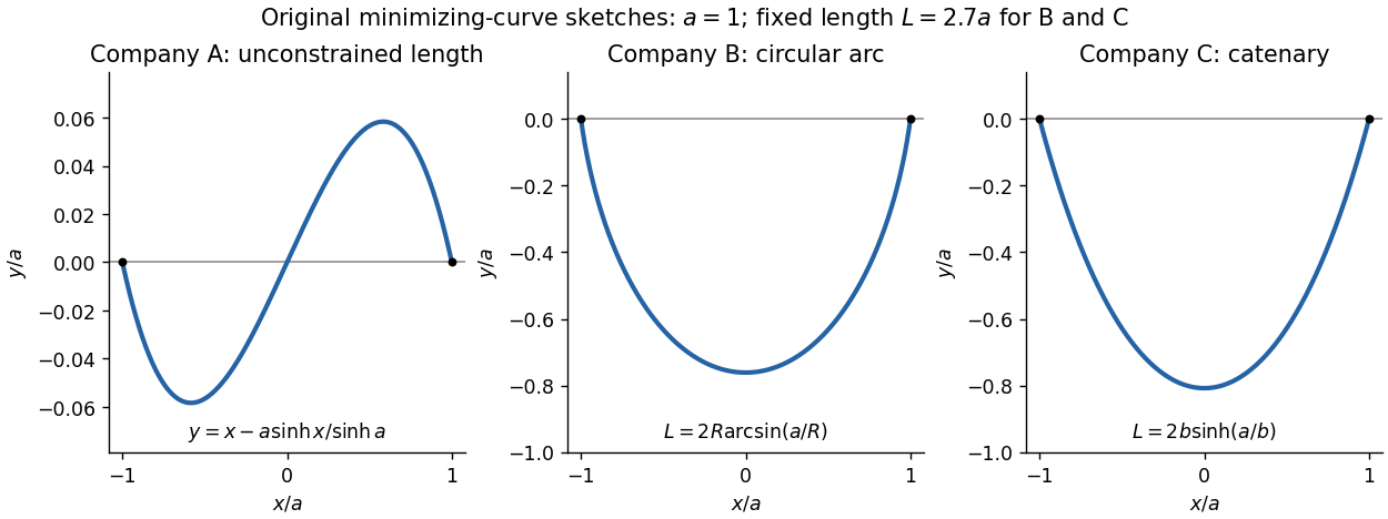
The sketch uses $a=1$ and $L=2.7$ for the two fixed-length cases. The vertical scale in the company A panel is enlarged to show its small odd deflection. No comparison between the three companies' absolute prices is required or possible from the shapes alone, since their additive cost constants are independent.

When $r=p^{\prime }$, write the differential expression in divergence form,Two integrations by parts give the Lagrange identity for a Sturm-Liouville operator:The $q$ terms cancel because $q$ is real. Hence the exact boundary criterion, in the sense of self-adjointness defined in the question, isAt regular endpoints, all separated homogeneous conditions of the following type satisfy it:with real coefficients, not both zero at either endpoint. The allowed value-and-flux pairs at an endpoint are proportional, so their determinant $p(f{g}^{\prime }-f^{\prime }g)$ vanishes. This includes Dirichlet boundary conditions, Neumann boundary conditions, Robin boundary conditions and arbitrary mixtures of these at the two ends.

Coupled conditions can also work: periodic conditions $y(b)=y(a)$ and $p(b)y^{\prime }(b)=p(a)y^{\prime }(a)$ make the two endpoint expressions equal; simultaneous minus signs give the antiperiodic case. Thus requiring each endpoint term separately to vanish is sufficient, but not necessary.

More generally, for regular endpoints set $Y=(y(a),y(b){)}^{\mathsf{T}}$ and $N=(-p(a)y^{\prime }(a),p(b)y^{\prime }(b){)}^{\mathsf{T}}$. All maximal homogeneous self-adjoint boundary conditions can be written $AY+BN=0$ with real two-by-two matrices satisfying $\mathrm{rank}(AB)=2$ and $A{B}^{\mathsf{T}}=B{A}^{\mathsf{T}}$. If an endpoint is singular, the relevant limiting boundary form and admissible domain must instead be specified; the assumption $p>0$ only in the interior does not itself fix those endpoint limits.

First move the order parameter term to the right-hand side:Here $p=x^2$, $r=x$, so the integrating factor obeysChoose the irrelevant positive constant $C=1$. Multiplying the equation by $1/x$ givesThus a Sturm-Liouville theory eigenvalue formulation with the requested eigenvalue isThis is the Sturm-Liouville formulation with Bessel order as eigenvalue. The spectral parameter is the squared order of the Bessel function, with $\beta$ treated as fixed. This differs from the also familiar formulation in which ${\beta }^2$ is the eigenvalue.

The factor $1/x$ is singular at the origin. Consequently the integral defining $w$ cannot literally use lower limit zero; take a positive reference point $x_{\ast }>0$, obtain $w=x_{\ast }/x$, and absorb $x_{\ast }$ into the normalization. The differential identity holds for $x>0$. Boundary conditions and admissibility at zero and at the outer endpoint are additional ingredients needed to make a particular self-adjoint spectral problem.

Denote the unshifted differential expression by $L_{0}y=(p{y}^{\prime }{)}^{\prime }+qy$. The supplied Green's function satisfies $L_{0}G(x,\xi )=\delta (x-\xi )$, whereas the inhomogeneous equation is $L_{0}y=\lambda wy+wf$.

Multiply the latter equation by $G$ and the Green equation by $y$, subtract and integrate in $x$:The left-hand side is the boundary termIt vanishes because $G$ and $y$ satisfy the same homogeneous Robin boundary conditions. For example, where $\alpha \ne 0$, substituting $y^{\prime }=-\beta y/\alpha$ and $G_x=-\beta G/\alpha$ cancels the endpoint expression; where $\alpha =0$, both values vanish. The other endpoint works identically. HenceThe Dirac delta function contribution is valid for an interior evaluation point $\xi$; equivalently, $G$ is continuous there and has flux-derivative jump $[p{G}_x{]}_{{\xi }^{-}}^{{\xi }^{+}}=1$.

This uses the existence of the unshifted Green's function stated in the question. Such a function is not automatic for every choice of $p,q$ and endpoint conditions: a nontrivial zero mode of $L_0$ would obstruct an ordinary inverse and would require a compatibility condition and a modified Green's function. Under the stated inverse assumption, the differential equation and the displayed integral equation are equivalent for functions in the boundary-condition domain.

The Cauchy integral formula for derivatives, with $z_0=0$, givesThe derivative cycles of sine and cosine give ${\sin }^{(n)}(0)=\sin (n\pi /2)$ and ${\cos }^{(n)}(0)=\cos (n\pi /2)$. ThereforeIn particular the sine integral vanishes for even $n$, and the cosine integral vanishes for odd $n$. For the remaining cases their signs alternate. The radius is irrelevant provided $R>0$, since the numerator is entire and the origin is enclosed once counterclockwise.