Draw the Fabry–Pérot etalon with parallel mirrors and an incident beam making internal angle with their normal. Every emerging transmitted contribution has undergone one more internal round trip than its predecessor.
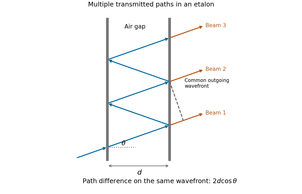

The extra internal path is , but successive contributions leave at laterally separated points, a distance apart. Comparing their phases on the same outgoing wavefront subtracts the path projection . Their net optical path difference in air isHence, in the reflection-phase convention implicit in the supplied transmission formula,For a gap of refractive index , replace by and use the vacuum wavelength. Coating reflection phases can add a round-trip offset; the expression above assumes that offset is absorbed in the resonance order, or is zero modulo as in the stated ideal model.
Write , keeping this coefficient distinct from the finesse . The transmission has maxima at . At a displacement from a maximum, its ratio to peak transmission is . Half maximum therefore requiresThis is the half-width in wave phase; the full width at half maximum is . Successive resonances are apart, so the exact ideal-model result isFor narrow peaks, , the small-angle approximation to the inverse sine givesThus the formula requested in the paper is the high-reflectivity approximation, not an exact identity at arbitrary . Ordinary half-maximum peaks exist only when , or ; below that threshold the transmission minimum never reaches half the peak. The prefactor cancels from this relative-width calculation.
Let , and . Requiring the separation to be at least times the measured full width at half maximum means a width no larger than , or a resolving power of approximately .
The etalon resolving power and order overlap constraints are particularly clear in frequency. Put . At normal incidence, the free spectral range is and the instrumental width is . ThusAvoiding ambiguity between the doublet and adjacent interference orders requires a free spectral range exceeding the doublet separation:Together these giveUsing the narrow-peak finesse from the previous part, gives , with a practical margin above that limiting value. At the exact limit, the gap between orders vanishes, so equality is not a sensible operating point.
One feasible ideal design is , , and . It has an approximate wavelength free spectral range of and instrumental width near the doublet. The doublet spacing is about widths. Even the spacing to the nearest replica of the other line exceeds widths in this example. If that latter separation is also required in general, impose the stronger condition , rather than just the two basic inequalities.
Such mirror reflectivities and submillimetre gaps are plausible for a high-quality Fabry–Pérot etalon. Flatness, parallelism, coating loss, angular spread, mechanical stability and source width limit the achieved finesse. A wavelength width of corresponds to a gap variation of order , so the ideal coating-limited estimate demands stringent uniformity. The paper expressly excludes intrinsic source broadening.
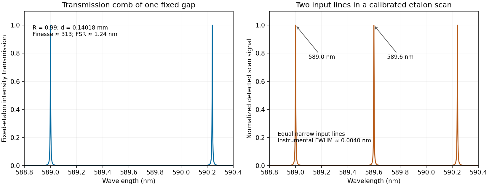
Calculated etalon transmission comb and a scanned doublet spectrum for an illustrative design meeting the width and order constraints
. Details. 
The first panel is the fixed etalon's transmission versus wavelength, a comb of resonances. It does not by itself have one peak at each sodium line. The second panel shows the two peaks obtained by scanning the etalon phase or gap and calibrating the scan to wavelength. A fixed-gap output spectrum is instead the incident spectrum multiplied by the transmission function. This distinction is needed to interpret a doublet measurement correctly.
A high-finesse Fabry–Pérot etalon obtains very narrow transmission peaks by summing many coherent round trips, allowing high resolving power with a compact optical path. It can transmit a substantial fraction of resonant light when coating absorption is small, and works well for precise relative line separations and narrow-line measurements. A diffraction grating may require many illuminated grooves to achieve the same resolving power.
The etalon's free spectral range is limited, and repeated orders cause ambiguity across a broad optical spectrum. It commonly needs scanning and an order-selecting optical filter or another dispersive element. Mirror alignment, flatness and illumination angle strongly affect peak positions and widths, and absorption lowers throughput. A diffraction grating instead separates a broad range of wavelengths spatially for simultaneous detection, although grating orders can also overlap. The preferred instrument depends on whether narrow-band precision or broad spectral coverage is the priority.
Here is displacement from equilibrium, in metres; is the oscillating mass, in kilograms; is the coefficient of linear viscous damping, in ; and is the spring constant, in . The terms , and are respectively the inertial term, the opposing velocity-dependent damping term and the opposing displacement-dependent restoring term when moved to the force side of Newton's second law.
is a possibly complex driving-force complex amplitude, measured in newtons. is the driving angular frequency in , and taking the real part of gives the physical sinusoidal force. Its frequency in hertz is . The natural undamped angular frequency and damping rate areThis damped harmonic oscillator model assumes a linear restoring force and a linear, instantaneous viscous damping law.
Set the drive to zero and try . The characteristic equation isFor underdamping, , the roots are , with . The displacement oscillates with an exponentially decaying envelope:For critical damping, , there is a repeated root , giving . The motion is nonoscillatory and is the limiting case between oscillatory and overdamped response.
For overdamping, , the roots are distinct negative real numbers and . Both components decay without sustained oscillation; strong damping gives a particularly slow late-time relaxation. Constants depend on the initial conditions. A nonoscillatory solution can cross equilibrium once for some initial data, so “nonoscillatory” does not mean monotone for every possible initial condition.
Let the initial conditions be and . The velocity-impulse response of a damped oscillator isAll curves start at the origin with the same positive slope . Underdamping gives a decaying sequence of positive and negative lobes. Critical damping gives one positive lobe followed by return to zero. Overdamping also remains positive for these initial data, but has a longer tail. The initial impulse changes velocity abruptly, not displacement.
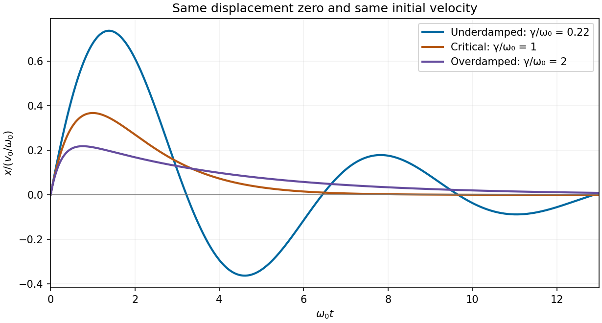
Calculated displacement after the same initial velocity impulse for underdamped, critically damped and overdamped oscillators
. Details. 
For underdamping, the general response is a free transient plus a particular driven response. Use the paper's convention. The steady displacement complex amplitude isThusHere , and the real constants enforce the initial conditions. For a real positive , the steady term is , whereFor light damping, and the transient decays slowly compared with an oscillation. The two-argument phase convention makes the displacement lag evolve from approximately zero below resonance through near to approximately far above it.
The response is quasistatic at low frequency, resonantly enhanced when the spring and inertia nearly cancel, and suppressed as at high frequency. The original graph gives approximate readings , and . These are graph estimates, not exact supplied measurements.
Use oscillator parameters from static and resonant displacement. The static spring constant isFor light damping, , givingNear resonance, , soIndependently, the resonance enhancement estimates the same quality factor. The half-power displacement level is ; its intersections are approximately and , giving bandwidth and .
The exact displacement-peak frequency is . At its difference from is only about , well below the precision justified by this printed curve. Greater numerical precision for the inferred parameters would be misleading.
In Fresnel diffraction, the propagation wave phase varies quadratically across the aperture and that curvature must be retained. For a transverse scale at propagation distance , its size is of order . In Fraunhofer diffraction, that quadratic term is negligible, approximately , while the linear phase encoding the observation angle remains. A lens can also form the far-field angular pattern in its focal plane.
For a normally incident plane wave and aperture transmission , the far-field complex amplitude is its Fourier transform:The detected light intensity is proportional to . For identical parallel slits, write the transmission as a sum of shifted copies of one slit. The Fourier shift theorem gives one single-slit transform multiplied by the sum of positional phase factors:The single-slit diffraction envelope sets the broad scale, while coherent interference between slit centres produces the finer array pattern. One sums complex amplitudes before squaring, rather than adding independent slit intensities.
Put the slit centres at . Each slit has the same width and illumination. Its contribution to the Fraunhofer diffraction complex amplitude isThe four phase factors pair into cosines:Therefore the four-slit Fraunhofer diffraction field isThe common factor can be absorbed in the proportionality constant, giving the requested form. In particular , as expected from four equal in-phase slits. Normalizing by the central intensity givesThe last form follows from and avoids apparent singularities in the usual sine-ratio array formula.
Let be horizontal position on the screen, , and use . The plotted interval is . With , and , the four-slit Fraunhofer diffraction intensity is the previous normalized expression evaluated at this angle. The total aperture width is , giving a Fresnel number of order , consistent with the far-field approximation.
Nominal principal array directions satisfy . Their screen positions areThus the visible nonzero orders are near , in addition to the central maximum. The even nonzero orders are missing diffraction orders: at the first envelope zero occurs at . The next envelope zero and direction lie at about , just beyond the screen edges.
At the nominal first and third array directions, and , respectively. The closest central minima satisfy , hence . Two small subsidiary array maxima occur between adjacent principal directions. The single-slit envelope slightly shifts the true off-axis maxima relative to the nominal principal array angles.
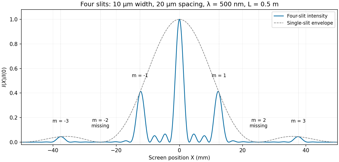
Calculated four-slit intensity across the specified screen, with principal array directions and missing orders marked
. Details. 
Model the two openings as identical axis-aligned rectangles of width in , height in , and centre separation along . Their Fraunhofer diffraction field has the formThe original image shows first broad envelope zeros near and . The horizontal interference period is about ; the first interference minima near distinguish that fine scale from the envelope. The rectangular-aperture dimensions from diffraction zeros are thereforeThe edge-to-edge gap is . The long direction is vertical. These dimensions also explain the suppressed alternate principal array maxima: .
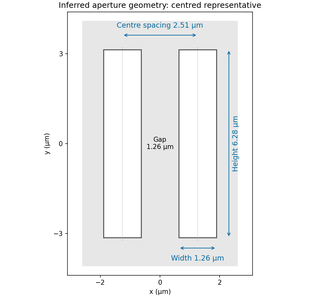
Inferred pair of rectangular openings, quantitatively labelled using the original angular-spatial-wavenumber axes
. Details. 
The factors are required by the stated convention; treating the plotted coordinates as cycles per micrometre would give different dimensions. The finite printed figure supports approximate dimensions. An overall translation and inversion of the aperture pair leave its Fourier intensity unchanged, so their absolute placement is not recoverable; the diagram chooses a convenient centred representative.
A waveguide confines the transverse structure of a wave while permitting propagation along a chosen route. It can deliver energy to a distant receiver without the same geometric spreading as an unguided beam, protect a signal from unwanted coupling, and select transverse normal modes. It also makes propagation paths and coupling to devices more controllable. Confinement does not eliminate wave absorption or scattering loss, and it can introduce wave dispersion and cutoff frequencies of a membrane waveguide or corresponding cutoffs for other wave types.
Two examples are an optical fiber, which guides light by its core-and-cladding refractive index structure, and a hollow electromagnetic waveguide used to carry microwaves between a source and an antenna. A duct for acoustic waves is a further example. Each uses different material and boundary conditions, but the common idea is controlled transverse confinement.
For the trial displacement , direct differentiation givesThe two-dimensional wave equation is therefore satisfied ifHere is the longitudinal wavenumber, the transverse wavenumber, and the speed of an unconstrained membrane wave. The physical displacement is the real part, multiplied by an arbitrary displacement amplitude. has units and is surface mass density in , so has units as required.
The fixed edge at is automatically satisfied by . At , the displacement must vanish at every , so . Thus the allowed transverse normal modes haveThe case gives zero displacement for this sine solution and is not a physical propagating mode. Negative only reverses the amplitude sign and does not create a distinct transverse mode. This discrete transverse spectrum is a consequence of the Dirichlet boundary conditions, rather than quantization of the longitudinal wavenumber in an indefinitely long guide.
For the th transverse mode, substitute into the membrane waveguide dispersion relation:Longitudinal propagation requires real nonzero , henceBelow the cutoff frequency of a membrane waveguide, , with , and a bounded excitation decays as rather than carrying a travelling wave along an infinite guide. At equality , the displacement has no longitudinal phase advance and the group velocity is zero; it is a cutoff oscillation, not a propagating mode carrying finite longitudinal power.
For positive angular frequency, the first three branches areEach branch is even in , has minimum , and starts with zero slope. At large , all approach the straight asymptote . Their group velocities are , whereas their longitudinal phase velocities are for , giving .
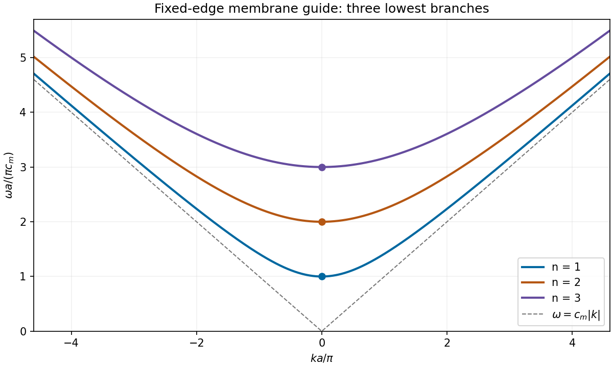
Three lowest membrane-waveguide dispersion branches, with their cutoffs and common large-wavenumber asymptote
. Details. 
Resistance to bending adds a restoring contribution that grows more rapidly with spatial curvature than the tension contribution. Short-wavelength modes are therefore stiffened especially strongly, raising their frequencies and changing the large-wavenumber behaviour.
For example, a thin plate of flexural rigidity has . When its edge conditions admit the same sine transverse mode, bending stiffness in a membrane waveguide givesThus the cutoffs increase, and bending-dominated propagation has at large , rather than approaching . Its phase velocity and group velocity then grow with . If “rigidly fixed” means a genuinely clamped plate edge, the slope must also vanish and the mode shapes change; the qualitative stiffening and stronger wave dispersion remain, but simple need not remain exact.
Articles by others on the same topic
There are currently no matching articles.