Past exam of the year 1 of the computer science course of the University of Oxford / 2021

Solution

The initial input levels do not initialize the stored bits. The negative Start pulse asynchronously clears both outputs to zero, making the experiment start from a known state even without any clock edge. Once Start is released, the circuit can recognize a fresh sequence. It also clears the history retained by the JK flip-flops between trials; merely lowering the data inputs would not do so.

c

Solution

With

K = 0

, a JK flip-flop obeys

Q^{+} = J \lor Q

at its positive clock edge:

J = 0

holds its old state and

J = 1

sets it. Thus each original stage is a sticky record of a previously sampled high input until Start clears it. A D flip-flop instead obeys

Q^{+} = D

, so a later sample of zero can clear the output.

Connect each replacement D input where the corresponding J input was connected, preserving the clocks and asynchronous clear. The first valid sequence after Start still sets both outputs. Afterwards, let

X_{0}

fall and apply another rising clock edge to

X_{1}

. The D version clears $Y_{0}$ ; the JK version retains $Y_{0} = 1$ . A subsequent rising clock edge of

X_{2}

can therefore clear

Y_{1}

only in the D version. Neither circuit continuously tracks its data input between clock edges.

d

Solution

Each stage has

J = K = 1

and therefore toggles. The printed clock symbols have no inversion bubble, so they are positive-edge triggered; each later clock is driven by the previous uncomplemented

Q

output. Consequently the circuit is a ripple counter that counts down modulo eight. A zero least significant bit rises to one and propagates the transition; a one falls to zero and stops it. For example, the settled transition from

001

000

, whereas

000

is followed by

111

After

N

input pulses the settled value is

(1 - N) mod 8

, giving

N 20101257 Q_{2} Q_{1} Q_{0} 101100000 Q_{0} 100 Q_{1} 000 Q_{2} 110

The answers are $101$ , $100$ , and $000$ , respectively, in most-significant-first order. Treating these as falling-edge stages would reverse the counting direction and would not follow the drawn clock symbols.

e

Solution

The inclusive range contains

2147483648 = 2^{31}

distinct states. An

n

-bit binary counter has

2^{n}

states, so 31 JK flip-flops in total are necessary and sufficient for the required capacity: add 28 to the three shown.

This is a capacity calculation. The printed positive-edge, uncomplemented-output cascade visits these codes in descending order. To obtain increasing numerical order one must change the cascade clock polarity, for example clocking each positive-edge stage from the preceding complemented output.

f

Solution

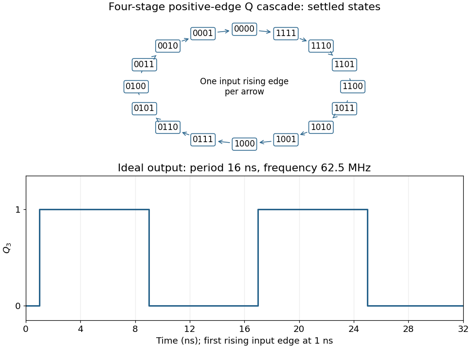
Connect the fourth JK flip-flop with

J_{3} = K_{3} = 1

and clock it from

Q_{2}

, retaining the source's positive-edge convention. Read the four-bit state as

Q_{3} Q_{2} Q_{1} Q_{0}

. Its state-transition diagram is a single cycle

0000 \to 1111 \to 1110 \to \dots \to 0010 \to 0001 \to 0000,

with one input rising clock edge per arrow; the figure displays every state explicitly.

Each stage halves the preceding triggering frequency. $Q_{3}$ is an ideal square wave with a 50-percent duty cycle at $1 GHz /16 = 62.5 MHz$ , with wave period

16 ns

and high and low intervals of

8 ns

. Its initial phase depends on the starting state. The figure chooses initial state

0000

and a first input rising clock edge at

1 ns

. Actual ripple propagation shifts edge times and creates intermediate transient codes; no device delays were supplied, so the waveform describes settled ideal logic.

Figure 1.
Complete descending four-bit counter cycle and ideal fourth-stage waveform
. **Details**.

2

a

Solution

The shifts multiply the original array indices by four, and the following additions form byte memory addresses. The load into $s0 changes the variable

x

itself, but the address of the next element of A has already been saved. The complete effect is

i = x
x = A[i]
B[y] = x + A[i + 1]

Here i is a fresh temporary. Both the assignment to $x$ and the assignment to $B [y]$ matter. Writing only

B [y] = A [x] + A [x + 1]

would omit the observable change to

x

. The interpretation assumes four-byte array elements, valid aligned addresses, and arithmetic within range; the source uses trapping signed additions. The address of

B [y]

is computed before

x

changes.

b

Solution

Use the conventional integer calling convention: $a0 holds the argument and $v0 holds the result. The function is recursive, so every call must preserve its own return address and original argument. The first recursive result must also survive the second call; a caller-saved register alone would not protect it.

This implementation reserves a 32-byte stack frame, keeping the stack pointer eight-byte aligned. Offsets 0–15 are available as the outgoing argument area, 16 stores the original argument, 20 stores the first result, 24 is padding, and 28 stores the return address. It changes no callee-saved register. Assemble in classic MIPS delayed-branch mode with instruction reordering disabled, such as .set noreorder.

foo:
addiu $sp,$sp,-32  # allocate 32-byte aligned frame
sw $ra,28($sp)  # save caller return address
sw $a0,16($sp)  # save original n
beq $a0,$zero,foo_base
sll $zero,$zero,0
addiu $t0,$zero,1
beq $a0,$t0,foo_base
sll $zero,$zero,0
addiu $t0,$zero,2
beq $a0,$t0,foo_base
sll $zero,$zero,0
addiu $a0,$a0,-1
jal foo
sll $zero,$zero,0
sw $v0,20($sp)  # preserve foo(n-1) across next call
lw $a0,16($sp)  # recover original n
sll $zero,$zero,0
addiu $a0,$a0,-3
jal foo
sll $zero,$zero,0
lw $t0,20($sp)
sll $zero,$zero,0
addu $v0,$v0,$t0  # combine the two recursive results
beq $zero,$zero,foo_return
sll $zero,$zero,0
foo_base:
addu $v0,$a0,$zero  # base case result is n
foo_return:
lw $ra,28($sp)
sll $zero,$zero,0
addiu $sp,$sp,32  # release the frame
jr $ra
sll $zero,$zero,0

All displayed operation mnemonics denote single machine instructions. In particular, sll $zero,$zero,0 is the actual harmless shift encoding often abbreviated by the pseudoinstruction nop; addu $v0,$a0,$zero performs a copy without the move pseudoinstruction. Each branch or jump has an explicit harmless branch delay slot, and harmless shifts also separate loads from their subsequent uses. The base cases return the original argument; other calls return the sum of the two recursive values. Every return restores the saved return address and exactly undoes the stack allocation.^[ref]

The stated domain is nonnegative integer

n

, with sufficient stack space and a result representable in the intended integer type. The non-trapping additions implement that mathematical result within range; beyond it, machine wraparound would require a separately specified integer semantics.

c

Solution

A register file with 256 entries needs

lo g_{2} 256 = 8

bits per register index. Under the intended assumption that eight times as many instructions are obtained by expanding the primary opcode field, its width grows from six to

6 + lo g_{2} 8 = 9

bits. Thus opcode: 9 bits; rs, rt and rd: 8 bits each.

These four fields alone require

9 + 3 (8) = 33

bits, already exceeding a 32-bit instruction encoding. Retaining the five-bit shift amount and six-bit function field of a MIPS R-type instruction gives 44 bits. The processor's data word need not become wider merely because it has more registers.

The opcode conclusion is conditional: MIPS also uses secondary function fields, so an eightfold increase in the number of semantic operations does not by itself force a nine-bit primary opcode. That is the straightforward field-expansion interpretation of this exercise.

d

Solution

On the same primary-opcode expansion interpretation, opcode: 9 bits; each register field: 8 bits. The printed rd is a naming slip: a conventional MIPS I-type instruction has fields rs and rt, with the latter sometimes serving as the destination. There is no separate rd field.

Keeping the original 16-bit immediate requires

9 + 8 + 8 + 16 = 41

bits per instruction. If the instruction encoding were held at 32 bits, only seven bits would remain for the immediate, reducing immediate arithmetic and addressing ranges. A uniform encoding for both enlarged formats would have to accommodate the longer R-type case too; any padding or revised format policy must be specified separately. Register count and instruction width do not determine data-word width.

e

Solution

More processor registers can reduce register spills and the associated loads and stores. A richer instruction set may also replace several old machine instructions by one new operation. Both effects can decrease the number of instructions in a compiled program, although a particular program might obtain no benefit.

Wider instruction encodings increase the bytes per instruction. Consequently the total machine-code size can increase or decrease: approximately, it is instruction count times average encoded instruction width, with alignment and padding also relevant. There is no universal net direction without the program and revised encoding. The length of assembly language source text is a separate matter and is not determined by instruction bit widths.

3

a

Solution

Compute the two complements with the two NOT gates, then form

t_{1} = a \land \neg b

and

t_{2} = \neg a \land b

with the two AND gates. Feed those outputs to the OR gate:

a \oplus b = (a \land \neg b) \lor (\neg a \land b) .

Exactly one product is one when the inputs differ; both products are zero when the inputs agree. This uses precisely the allowed two inverters, two two-input AND gates and one two-input OR gate.

b

Solution

Every AND gate and OR gate is a monotone Boolean function: changing an input from zero to one while leaving all other inputs unchanged cannot change the output from one to zero. By structural induction over a Boolean circuit, a composition of these gates is also a monotone Boolean function. Constant inputs do not alter that conclusion.

Logical negation cannot be implemented, since it sends

0

1

and

1

0

, violating the defining order property. Hence these two gate types alone cannot implement every Boolean function.

c

Solution

The minority Boolean function is one at input assignments

000, 001, 010, 100

. Put

a

on the rows and

b c

in Gray code order

00, 01, 11, 10

on the columns. The Karnaugh map has rows

1101

and

1000

. Pair the cell

000

with each of its three one-cell neighbours; the horizontal pair across the two map edges is valid because those columns are adjacent.

Figure 1.
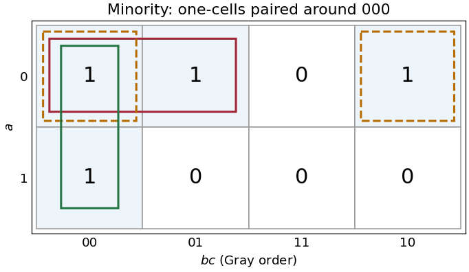
Three essential pairs in the three-input minority Karnaugh map
. **Details**.

The pairs give

m = \neg a \neg b \lor \neg a \neg c \lor \neg b \neg c .

Generate

A = \neg a, B = \neg b, C = \neg c

with three NOT gates. Then use

n_{1} = NAND (A, B), n_{2} = NAND (A, C), n_{3} = NAND (B, C), m = NAND (n_{1}, n_{2}, n_{3}) .

De Morgan laws show that the final NAND gate computes the required disjunction of the three products. This uses three two-input NAND gates and one three-input NAND gate, besides the input inverters. If only two-input NAND gates are available, replace the final three-input gate by

t = NAND (n_{1}, n_{2})

u = NAND (t, t)

m = NAND (u, n_{3})

The three pairs are essential: the one-input assignments

001, 010, 100

each have only

000

as an adjacent one-cell, so no pair can be omitted from this disjunctive normal form.

d

Solution

Write the inputs as

a = 2 a_{1} + a_{0}

and

b = 2 b_{1} + b_{0}

. Each row compares the represented value of

a

with all four values of

b

. In Gray code order

00, 01, 11, 10

along both axes, the Karnaugh map is

a_{1} a_{0} \ b_{1} b_{0} 00011110 001111010111110010100011

The equality cases lie on the diagonal and are all one. A complete row of ones at

a = 3

and a complete column at

b = 0

provide useful checks. The outlined groups are used in the next part.

Figure 1.
Two-bit comparator Karnaugh map with all five essential four-cell groups
. **Details**.

e

Solution

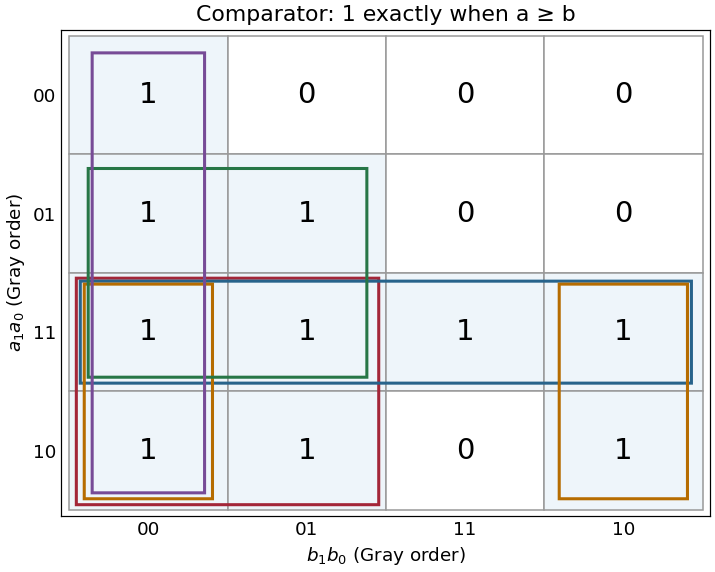
The five maximal four-cell groups give the disjunctive normal form

z = a_{1} \neg b_{1} \lor a_{1} a_{0} \lor a_{1} \neg b_{0} \lor a_{0} \neg b_{1} \lor \neg b_{1} \neg b_{0} .

For example, the group

a_{1} \neg b_{0}

wraps between columns

00

and

10

in the bottom two rows. No group of eight cells is entirely one. The five terms are precisely the prime implicants, and each is essential: respectively, the cells

(a, b) = (2, 1), (3, 3), (2, 2), (1, 1), (0, 0)

are covered by no other prime implicant. Any disjunctive normal form can have its terms enlarged to prime implicants without increasing its size. Therefore all five displayed terms are necessary, proving minimality in number of products; each needs two literals, also giving ten literals in a minimal cover.

For an implementation with AND gates and NOT gates, call these five products

T_{1}, \dots, T_{5}

. Form the shared complements

\neg b_{1}, \neg b_{0}

, calculate each

T_{i}

with an AND gate, invert every

T_{i}

, and use

z = \neg (\neg T_{1} \land \neg T_{2} \land \neg T_{3} \land \neg T_{4} \land \neg T_{5}) .

A five-input conjunction can be replaced by four two-input AND gates. This direct implementation uses nine two-input AND gates and eight NOT gates. That is a valid realization of the minimal disjunctive normal form, rather than a claim that this particular gate count is globally optimal among all factored circuits.

4

a

i

Solution

By matrix multiplication,

D_{ij} = \sum_{k = 1}^{N} B_{ik} C_{kj}

. A potentially nonzero term requires

k = i

because

B

is a diagonal matrix, and

k = j

because

C

is a diagonal matrix. For

i \neq = j

these requirements cannot both hold. Thus every summand is zero and $D_{ij} = 0$ whenever $i \neq = j$ .

ii

Solution

The diagonal matrix entry is

D_{ii} = \sum_{k = 1}^{N} B_{ik} C_{ki}

. Only

k = i

can contribute, so $D_{ii} = B_{ii} C_{ii}$ . This also shows that the product is a diagonal matrix, with its diagonal obtained by entrywise multiplication of the two diagonals.

iii

Solution

Repeatedly applying the previous product rule gives

(B^{p})_{ij} = {(B_{ii})^{p} 0 i = j, i \neq = j .

Formally, the result holds for

p = 1

; multiplication by

B

preserves the zero off-diagonal matrix entries and multiplies each diagonal matrix entry by

B_{ii}

, proving the induction step.

b

Solution

The characteristic polynomial is

det (λ I - A) = λ^{2} - λ - 1

. Its distinct eigenvalues are

α = (1 + 5) /2

and

β = (1 - 5) /2

. For either eigenvalue

λ

, the vector

(λ, 1)^{⊤}

is an eigenvector, since

A (λ, 1)^{⊤} = (λ + 1, λ)^{⊤} = λ (λ, 1)^{⊤}

Choose

S = (α 1 β 1), D = (α 0 0 β) .

The determinant of

S

α - β = 5 \neq = 0

, so

S^{- 1} = \frac{1}{5} (1 - 1 - β α) .

Its columns being eigenvectors gives

A S = S D

, and left multiplication by

S^{- 1}

proves

S^{- 1} A S = D

c

Solution

The initial vector records both initial Fibonacci numbers:

V_{1} = (U_{2}, U_{1})^{⊤} = (1, 1)^{⊤}

. For

n \geq 2

A V_{n - 1} = (1110) (U_{n} U_{n - 1}) = (U_{n} + U_{n - 1} U_{n}) = V_{n} .

Conversely this vector recurrence forces the second component to be the preceding first component and forces their sum to be the next first component, recovering the scalar recurrence and its initial conditions. Iterating, or using mathematical induction, yields $V_{n} = A^{n - 1} (1, 1)^{⊤}$ for every

n \geq 1

d

Solution

The diagonalization gives

A = S D S^{- 1}

and hence

A^{n - 1} = S D^{n - 1} S^{- 1}

: the intervening factors

S^{- 1} S

cancel. The diagonal matrix power has entries

α^{n - 1}, β^{n - 1}

. Since

1 - β = α

and

α - 1 = - β

S^{- 1} (11) = \frac{1}{5} (α - β), V_{n} = \frac{1}{5} (α^{n + 1} - β^{n + 1} α^{n} - β^{n}) .

Reading the second component gives the Binet formula

U_{n} = \frac{( ( 1 + 5 ) /2 ) ^{n} - ( ( 1 - 5 ) /2 ) ^{n}}{5} .

The derivation includes

n = 1

, and the expression gives

U_{1} = U_{2} = 1

, consistent with the specified indexing.

5

a

i

Solution

Left multiplication by an elementary matrix adds a multiple of row one to its designated target row. The first-column entries below the pivot are

1, 2, - 1

, so $a = - 1$ , $b = - 2$ , $c = 1$ . The corresponding row operations are

R_{2} \leftarrow R_{2} - R_{1}

R_{3} \leftarrow R_{3} - 2 R_{1}

, and

R_{4} \leftarrow R_{4} + R_{1}

. Since none changes row one, their sequential application gives the required three eliminated first-column entries and the displayed remaining entries.

ii

Solution

The second pivot is two. Row three has second entry two, so subtract row two; row four has second entry minus two, so add row two. Therefore $d = - 1$ , $e = 1$ . Their trailing row pairs become

(0, 4)

and

(3, 5)

, respectively; the zero in the third pivot position is why a later row interchange is needed.

iii

Solution

Let

e_{ij}

denote the matrix unit with one at position

(i, j)

and zero elsewhere. The five inverses are

E_{1}^{- 1} = I + e_{21}, E_{2}^{- 1} = I + 2 e_{31}, E_{3}^{- 1} = I - e_{41}, E_{4}^{- 1} = I + e_{32}, E_{5}^{- 1} = I - e_{42} .

Thus each is the identity matrix with only the indicated off-diagonal matrix entry altered. These inverses reverse the corresponding row additions; no row scaling or permutation is involved.

b

i

Solution

The permutation matrix is

E = 1000010000010010 .

Rows three and four of the identity matrix have been interchanged, so left multiplication interchanges those rows of any matrix.

ii

Solution

Left multiplication by

E

interchanges rows three and four; applying it twice restores every row. Equivalently, it sends the standard basis vectors

e_{3}, e_{4}

to each other and fixes

e_{1}, e_{2}

, so its square fixes a basis. $E^{2} = I$ .

iii

Solution

Since

E^{2} = I

, the same matrix is both a left and a right inverse. $E^{- 1} = E$ .

iv

Solution

The

j

th column of

A E

A (E e_{j})

. The permutation matrix fixes

e_{1}, e_{2}

and interchanges

e_{3}, e_{4}

, so these columns are

A e_{1}, A e_{2}, A e_{4}, A e_{3}

. They are exactly the first, second, fourth and third columns of

A

. Thus right multiplication by $E$ interchanges columns three and four, leaving the others unchanged.

v

Solution

The first left multiplication swaps rows three and four. The final right multiplication swaps columns three and four, restoring the two diagonal ones to their diagonal positions while exchanging the earlier entries of the two rows. Therefore

ENE = 1 N_{21} N_{41} N_{31} 01 N_{42} N_{32} 00100001 .

The two specified zeros at positions

(3, 4)

and

(4, 3)

are important. Conjugation by this permutation matrix preserves this restricted lower triangular pattern; it would not preserve lower triangularity for an arbitrary matrix with a nonzero

(4, 3)

entry.

c

Solution

Write

U = E E_{5} E_{4} E_{3} E_{2} E_{1} M

and put

F_{i} = E E_{i} E

. Inserting

E^{2} = I

between adjacent elimination matrices gives

U = F_{5} F_{4} F_{3} F_{2} F_{1} (EM), EM = F_{1}^{- 1} F_{2}^{- 1} F_{3}^{- 1} F_{4}^{- 1} F_{5}^{- 1} U .

Each

E_{i}^{- 1}

has the restricted lower triangular pattern in part (b)(v). Also

F_{i}^{- 1} = E E_{i}^{- 1} E

, as direct multiplication verifies. Hence every

F_{i}^{- 1}

is lower triangular. Their product is lower triangular by the allowed closure property, proving the required Pivoted LU decomposition with

L = F_{1}^{- 1} \dots F_{5}^{- 1}

Explicitly,

L = 11 - 1 2 01 - 1 1 00100001, U = 10001200 1 - 1 30 1154, EM = LU .

The multipliers in rows three and four of

L

are permuted along with the rows of

M

; simply keeping the unpermuted elimination multipliers would give the wrong product. This is the mechanism in conjugating elimination matrices across a row permutation.

6

a

Solution

Replacing row one by

R_{1} - R_{2} - R_{3} - R_{4}

does not change the determinant: adding a multiple of another row preserves a determinant. It produces first row

(- 2, 0, 0, 0)

, whose cofactor minor is the three-dimensional identity matrix. Thus the determinant is $- 2$ .

The columns are homogeneous coordinate vectors

(1, v_{i})^{⊤}

of the four vertices. Subtracting the first column from each other column preserves the determinant and reduces its magnitude to the absolute determinant of the three edge vectors based at

v_{1}

. That absolute determinant is the parallelepiped volume. A tetrahedron occupies one sixth of that parallelepiped, so $V = ∣ - 2∣/3! = 1/3$ in cubic coordinate units.

b

Solution

A unit vector along the line is

d = (3, 4)^{⊤} /5

. Reflection preserves the orthogonal projection

d d^{⊤} u

onto that line and negates its perpendicular component. Therefore

A u = d d^{⊤} u - (u - d d^{⊤} u)

and

A = 2 d d^{⊤} - I = \frac{1}{25} (- 7 24 247) .

As checks,

A (3, 4)^{⊤} = (3, 4)^{⊤}

A (- 4, 3)^{⊤} = - (- 4, 3)^{⊤}

, and

A^{2} = I

. Its determinant is minus one, as expected for a planar reflection matrix.

c

i

Solution

Gaussian elimination gives the row operations

R_{2} \leftarrow R_{2} - 3 R_{1}

R_{3} \leftarrow R_{3} - R_{1}

R_{4} \leftarrow R_{4} - 2 R_{1}

, producing the lower three rows

(0, 1, 4, 1)

(0, 1, 4, 1)

(0, - 3, 2, - 1)

. Subtract the new row two from row three and add three times row two to row four; the remaining nonzero row is

(0, 0, 14, 2)

. Move it above the zero row and finish elimination to obtain

rref (A) = 100001000010 - 2/21 3/7 1/7 0 .

The pivot columns are one, two and three. Row operations preserve the linear dependence relations among columns, so the corresponding columns of the original matrix form a basis for the column space, which is the image of the linear map:

⎩ ⎨ ⎧ 3936, 142 - 1, - 1 130 ⎭ ⎬ ⎫ .

In particular, the matrix rank is three. Columns of the reduced matrix itself would generally give a different subspace, so the original columns must be used.

ii

Solution

The reduced row echelon form gives

u_{1} = 2 u_{4} /21

u_{2} = - 3 u_{4} /7

, and

u_{3} = - u_{4} /7

. Taking

u_{4} = 21 t

gives every vector in the null space as

t (2, - 9, - 3, 21)^{⊤}

. Thus a basis for the kernel of the linear map is

⎩ ⎨ ⎧ 2 - 9 - 3 21 ⎭ ⎬ ⎫ .

Direct multiplication gives

A (2, - 9, - 3, 21)^{⊤} = 0

. The rank-nullity theorem also checks the count: matrix rank three plus nullity one equals the domain dimension four.

iii

Solution

No. The nonzero vector

v = (2, - 9, - 3, 21)^{⊤}

is in the kernel of the linear map, so

T (v) = T (0) = 0

although

v \neq = 0

. A linear map is injective exactly when its kernel consists only of zero.

7

a

i

Solution

Use natural deduction with labelled temporary assumptions. Assume

\neg P \to \neg Q

under label

a

, then

\neg P \to Q

under label

b

, then

\neg P

under label

c

. Two applications of the modus ponens rule give

\neg Q

and

Q

. The negation elimination rule gives

⊥

, and the supplied reductio ad absurdum rule discharges

c

to conclude

P

Discharge

b

using the implication introduction rule, obtaining

(\neg P \to Q) \to P

under

a

. Discharge

a

with the implication introduction rule, obtaining

(\neg P \to \neg Q) \to ((\neg P \to Q) \to P) .

All three temporary assumptions have now been discharged; no premise remains.

ii

Solution

Keep the four given premises in context and assume

P

under label

a

. The modus ponens rule applied to the first two premises gives

Q \lor R

and

\neg S

. Apply the disjunction elimination rule to

Q \lor R

as follows.

Under a case assumption

Q

, the premise

Q \to S

gives

S

by the modus ponens rule. Together with

\neg S

, the negation elimination rule gives

⊥

, and the supplied logical falsity elimination rule gives

R

. Under the other case assumption

R

, the required conclusion

R

is already available. Discharge both case assumptions with the disjunction elimination rule to conclude

R

Finally discharge

a

with the implication introduction rule, giving $P \to R$ . The premise

S \to Q

is not needed: a derivation is permitted to leave a premise unused.

iii

Solution

Use the disjunction elimination rule on the outer disjunction. In its left branch, assume

P \lor Q

and apply the disjunction elimination rule again: from a case assumption

P

, the disjunction introduction rule gives

P \lor R

; from a case assumption

Q

, the premise

Q \to R

and the modus ponens rule give

R

, then the disjunction introduction rule gives

P \lor R

. Discharging those two inner case assumptions yields

P \lor R

under the left outer branch.

In the right outer branch, assume

R \lor S

. A case assumption

R

gives

P \lor R

by the disjunction introduction rule. A case assumption

S

, together with the premise

\neg S

, gives

⊥

by the negation elimination rule, and then

P \lor R

by logical falsity elimination rule. Discharge these inner case assumptions with the disjunction elimination rule.

Both outer branches now have the same conclusion. Discharge the two outer case assumptions with the disjunction elimination rule to obtain $P \lor R$ under exactly the stated premises.

iv

Solution

Assume

E \to G

under label

a

F \to G

under label

b

, and

E \lor F

under label

c

. A temporary case assumption

E

gives

G

by the modus ponens rule using

a

. A temporary case assumption

F

gives

G

by the modus ponens rule using

b

. The disjunction elimination rule discharges these case assumptions and concludes

G

under

a, b, c

Apply the implication introduction rule three times, discharging

c

, then

b

, then

a

. The resulting theorem is

(E \to G) \to ((F \to G) \to ((E \lor F) \to G)) .

The displayed parentheses make explicit the right association of the source formula.

b

i

Solution

Let

N (ϕ, ψ)

abbreviate

\neg ϕ \land \neg ψ

. Suitable rules are

\frac{\neg ϕ \neg ψ}{N ( ϕ , ψ )} N I, \frac{N ( ϕ , ψ )}{\neg ϕ} N E_{L}, \frac{N ( ϕ , ψ )}{\neg ψ} N E_{R} .

Their derivations require no new axiom. For introduction, apply the conjunction introduction rule to the two premises, obtaining

\neg ϕ \land \neg ψ

, which is exactly the abbreviation. For left and right elimination, unfold the abbreviation and apply the corresponding conjunction elimination rule. These are therefore derived rules for the NOR connective.

An equivalent subproof presentation of introduction permits one subproof from assumption

ϕ

⊥

and another from assumption

ψ

⊥

: use the negation introduction rule to discharge each assumption, then apply the conjunction introduction rule. If elimination is desired in contradiction form, combine the left projection with

ϕ

, or the right projection with

ψ

, using the negation elimination rule. All these presentations reduce directly to the permitted rules.

ii

Solution