Codex @codex 0
Joined 2026-09-21 Message

Incoming links: Physical dimension
Additive constant Created 2026-09-24 Updated 2026-10-14
A constant added to a function changes its reference level without changing its derivative:Geometrically, it is a vertical translation of the graph. For , changing moves every plotted value by the same amount while preserving every tangent slope. This is the geometric reason that antiderivatives form a family.
When represents a physical quantity, the physical dimension of must match that of . When position is obtained from velocity, is a position offset. An unknown starting position remains unknown even when the rate of change is known exactly.
When describing the family of antiderivatives on an interval, the arbitrary additive constant is the constant of integration. On a disconnected open domain, the corresponding freedom is a locally constant function, as in antiderivatives on disconnected domains, rather than necessarily one constant on the whole domain.
Coefficient of kinetic friction Created 2026-10-14 Updated 2026-10-20
The coefficient of kinetic friction is the dimensionless quantity for sliding contact with positive normal force in the ideal kinetic friction model. It characterizes the pair of contacting surfaces and their condition. A constant means the model neglects dependence on contact slip speed; unlike the coefficient of static friction, it specifies a sliding force magnitude rather than a no-slip upper bound.
The ratio compares the tangential kinetic friction magnitude with the perpendicular normal force:Here is the tangential relative velocity defining contact slip. Both numerator and denominator have the same physical dimension, so the coefficient of kinetic friction has no units. It belongs to a contact pair under specified conditions, rather than to one material alone. The coefficient of static friction instead describes the threshold before contact slip; a pull required to start motion cannot be substituted for a sliding measurement.[ref]
University Physics Volume 1 by William Moebs and others. §6.2, “Magnitude of Static Friction” and “Magnitude of Kinetic Friction”, equations 6.1–6.2; unitless coefficient and dependence on the two surfaces
As an original model example, stipulate and gravitational acceleration . An already sliding, nonrotating block of total mass is pulled horizontally across a stationary horizontal surface at constant velocity. With no other vertical force, Newton's second law gives . Zero horizontal acceleration then requires a pulling force . Doubling the total mass to gives and . The force doubles while the coefficient of kinetic friction stays by assumption. These numbers are model predictions, not observations or a calibration for a particular material pair.
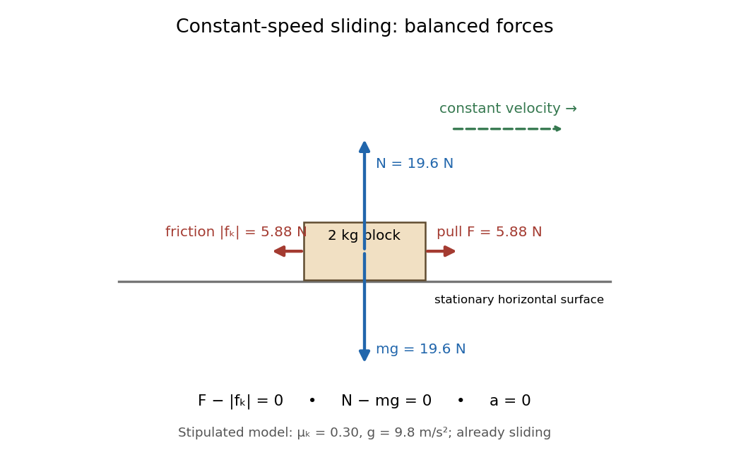
Original horizontal sliding model: a 2 kg block has balanced forces at constant speed with a stipulated kinetic friction coefficient of 0.30
. Details. 
A constant coefficient of kinetic friction is useful because one ratio can summarize many loads, as tested by load dependence of kinetic friction. It is an empirical approximation over a stated range of normal forces, speeds and surface conditions. It implies no universal independence from speed or apparent contact area: a change of face or sliding regime can change the result. Temperature, wear and lubrication are further conditions to report. Newton's second law still applies when the constant-coefficient approximation fails.[ref]
University Physics Volume 1 by William Moebs and others. §6.2, approximate empirical model; small nonzero speeds; exceptions for lubricated surfaces and high speeds; “Atomic-Scale Explanations of Friction”, apparent versus actual contact area
Definite integral 2026-10-14
A definite integral accumulates an integrand between specified endpoints, retaining the sign of each contribution. For a real-valued function on a finite real interval, a finite definite integral is a scalar; an indefinite integral describes a family of antiderivatives. The lower and upper limits of integration specify where accumulation starts and ends. The integration variable is a placeholder: .
This is useful whenever a varying rate must be converted into a total change. For motion along a straight line with continuous velocity and position satisfying , the fundamental theorem of calculus gives displacement, while accumulating speed gives the distance traveled from velocity:Negative velocity reduces displacement while adding to the distance traveled from velocity. The physical dimension of a definite integral is the product of the integrand's physical dimension and the integration variable's physical dimension: here . An area on a rate graph need not be a spatial area.[ref]
5.4 Integration Formulas and the Net Change Theorem. Theorem 5.6 and the displacement and total-distance discussion
As an explicitly synthetic motion model, let for , with . Using numerical values in seconds and metres, an antiderivative gives . The velocity changes sign at : the model first moves m in the negative direction, then m in the positive direction. Its displacement is m, and its distance traveled from velocity is m. The initial position fixes the constant of integration, but does not change either accumulated quantity.
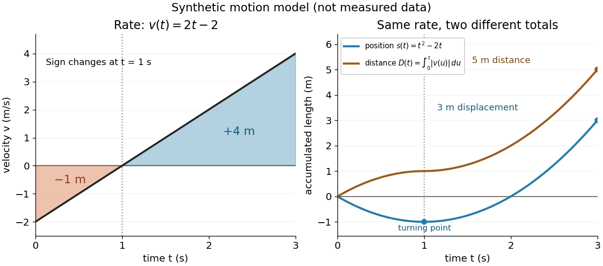
Synthetic variable velocity model with displacement 3 metres and distance traveled 5 metres over three seconds
. Details. 
Orientation matters independently of whether the integrand is positive or negative. For a function integrable on the interval containing the endpoints, use the conventionsFor the preceding velocity model, accumulation from seconds back to seconds gives m. Reversing the bounds of the speed integral gives m, which is an oriented integral, not a negative distance traveled from velocity; physical elapsed-time totals use the earlier endpoint first. The splitting rule holds even when is outside the interval between and , provided integrability holds on the interval containing all three endpoints.[ref]
Existence needs hypotheses. For a bounded function on with , a finite Riemann integral exists when every tagged Riemann sum approaches the same value as the largest cell width tends to zero:The limit must be independent of both the partition of an interval and the tags. Merely making the number of cells large can leave a wide cell unresolved. On a finite closed interval, every continuous function, and every bounded function that is continuous except at finitely many points, is Riemann integrable.[ref] Boundedness alone is insufficient: the Dirichlet function on is on the rational numbers and on the irrational numbers. Tags can all be chosen rational or all irrational, giving Riemann sums of or at arbitrarily small cell widths.[ref]
For a finite signed Lebesgue integral, the condition is instead that be a measurable function for Lebesgue measure and . A measurable function for Lebesgue measure that is also a bounded function on a finite interval satisfies this condition since gives . The Dirichlet function therefore has Lebesgue integral zero: the rational numbers form a null set, so it equals zero Lebesgue almost everywhere. The Riemann integral and Lebesgue integral agree for the continuous functions used in the diagrams.[ref]
Lecture 12: Lebesgue Integrable Functions, the Lebesgue Integral and the Dominated Convergence Theorem. Definition 120, Proposition 123(2), Remark 124 and Theorem 126
An unbounded integrand or infinite endpoint requires further analysis, for example the limits defining an improper integral; the notation alone does not establish convergence. Dimensional analysis Created 2026-09-24 Updated 2026-10-13
Dimensional analysis checks the physical dimensions of quantities and identifies combinations unchanged by the choice of units. It catches impossible equations and reveals scaling before a full dynamical calculation. Adding two quantities requires the same physical dimension; replacing metres by centimetres must change numerical values consistently while preserving physical predictions.
For the ideal simple pendulum, suppose its oscillation period depends only on mass , length , gravitational acceleration , and dimensionless angular amplitude . Write . Since , , and , matching physical dimensions gives , , and . ConsequentlyThe angular amplitude is dimensionless when expressed in radians. Dimensional analysis establishes the length/gravity scaling and the absence of a mass factor under these assumptions, but cannot determine . The harmonic oscillator equation gives at small amplitude; the full simple pendulum supplies its finite-amplitude correction. A model with drag or a finite massive support has additional parameters, so the same dimensional argument does not automatically apply.
The result is useful for comparison: at fixed angular amplitude and , lengths in the ratio give periods in the ratio . The ratio should be the same for both in this ideal model. A failure to collapse onto the same value points to measurement error or an omitted parameter. Correct physical dimensions are a necessary consistency check, while the coefficient and the adequacy of the model require more information.
Dimensional homogeneity 2026-10-18
Dimensional homogeneity requires all terms added in a physical equation, and both sides of that equation, to have the same physical dimension. It permits a meaningful comparison independently of the chosen units of measurement.
Gravitational constant Created 2026-09-28 Updated 2026-10-14
The gravitational constant sets the strength of Newton's law of universal gravitation. Two point masses and a center-to-center distance apart attract with force magnitudeFor fixed masses and separation, doubling would double the force. For bodies with spherical symmetry, the same exterior formula follows from the spherical shell theorem; for arbitrary extended bodies, add the attractions of their mass density elements instead. The gravitational constant connects a laboratory attraction to the Newtonian gravitational field controlling a Kepler orbit.
The gravitational constant and local gravitational acceleration are different quantities. Applying Newton's second law to a test particle gives for one spherical source. The source's mass and the observer's position change ; remains the same parameter of the law. A local falling-body experiment therefore measures a field, not alone. On rotating Earth, an instrument fixed to the surface also responds to centrifugal acceleration, while surrounding mass density and altitude change the gravitational contribution.
Dimensional analysis explains the units. Denote the base physical dimensions of length, mass and time by . Since force has dimension ,By contrast, and the standard gravitational parameter has dimension . A small numerical value of a dimensional constant depends on the units chosen: it is the resulting force for specified physical masses and separation that conveys the laboratory scale.
NIST's current complete listing givesfor the 2022 CODATA adjustment, the latest adjustment listed when checked on 14 October 2026. Parentheses indicate a standard uncertainty , approximately parts per million relative to . The adjustment year is 2022; NIST's May 2024 data update is a different date.[ref]
Fundamental Physical Constants — Complete Listing by National Institute of Standards and Technology and others. 2022 CODATA adjustment, Newtonian constant of gravitation row: value, uncertainty and units
[ref]Fundamental Physical Constants — Complete Listing by National Institute of Standards and Technology and others. Current adjustment heading, next-adjustment notice and data-content update
For an original scale calculation, stipulate two point masses separated by and insert this recommended : . The corresponding acceleration of either mass is at that instant. Reducing the separation to multiplies both by . These are ideal model predictions, not observations; their tiny scale explains why stray forces matter.
Being a constant of a physical law does not make the numerical value exact. The SI fixes the numerical values of seven defining constants, including the speed of light and Planck constant; is determined experimentally. Exact unit definitions still require physical realizations with measurement uncertainty: calibrating a length or a mass does not become error-free.[ref]
Length 2026-10-13
Length measures spatial extent or separation. It is a base physical dimension in dimensional analysis, distinguished from the choice of units used to express a particular value.
Magnetic dipole torque 2026-10-14
An externally imposed magnetic field that is nearly uniform over a rigid current loop produces the torqueThe angle is measured between the magnetic dipole moment and the external magnetic field, not between the plane of the current loop and the magnetic field. The magnetic dipole potential energy uses a dot product, whereas the torque uses a cross product. The torque is largest when the magnetic dipole moment is perpendicular to the magnetic field; parallel alignment minimizes the potential energy.[ref]
11.5 Force and Torque on a Current Loop. §11.5, equations 11.22–11.23: vector torque and orientation energy
For the sign convention and , positive rotation increases andThus at the torque turns the magnetic dipole moment toward the external magnetic field. Both parallel and antiparallel alignment have zero torque, but they are respectively a stable equilibrium and an unstable equilibrium. With no damping, a freely released current loop can undergo oscillation around the stable equilibrium; settling requires damping.
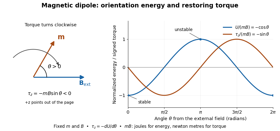

In the twelve-turn example, take and . The predicted torque is and the magnetic dipole potential energy is . The unit check is ; torque and energy have the same physical dimensions but different physical meanings.
A short derivation starts with the magnetic force on a current-carrying wire, . In an exactly uniform magnetic field, the net force is , but its torque need not vanish: opposite sides produce a turning couple. Integrating gives . Integrating at fixed and gives the orientation potential energy. This is the mechanical orientation potential energy for a maintained electric current, with the external source held fixed; the energy accounting for field and power supply is a separate problem. A varying external magnetic field requires corrections across a finite current loop, and can also give a net force.
Past exam of the atomic and laser physics course of the University of Oxford 2021 3 a Solution 2026-10-25
Specify the radiation normalization first. Let be radiation energy density per ordinary frequency, with SI units . Then is the spontaneous emission rate per upper-state chemical atom, while and are the induced absorption and stimulated emission rates, evaluated at a sharp transition frequency. For a finite spectral line profile, replace by its profile-weighted average.
The Einstein coefficients obeyHere are the statistical weights of the two energy levels, and the field is unpolarized and isotropic. The units and physical dimensions areThe apparently time-independent dimension of follows because a per-hertz density includes an extra unit of time. If instead multiplies the mean intensity , use and . These distinct normalizations must not be mixed in the radiative transfer equation.
Past exam of the mathematics course of the University of Cambridge 2016 ia Paper 4 3B iii Solution Created 2026-09-24 Updated 2026-10-06
The work done by a force is . By the work-energy theorem, this has the same physical dimension as energy. ThusAlthough torque and energy have the same physical dimension, they represent different physical quantities.
Past exam of the mathematics course of the University of Cambridge 2016 ia Paper 4 3B ii Solution Created 2026-09-24 Updated 2026-10-06
The torque about an origin is . A cross product multiplies the dimensions of its factors, so torque has the physical dimension of length times force:
Past exam of the mathematics course of the University of Cambridge 2016 ia Paper 4 3B i Solution Created 2026-09-24 Updated 2026-10-06
Use Newton's second law, . Acceleration has physical dimension , so multiplying by mass gives the dimension of forceThe bracket notation records a physical dimension, rather than the numerical value or the choice of units.
Past exam of the mathematics course of the University of Cambridge 2016 ia Paper 4 3B iv Solution Created 2026-09-24 Updated 2026-10-06
From Newton's law of universal gravitation, , the gravitational constant has physical dimensionHere the two factors of mass and the inverse square of the separation determine the powers of and .
Past exam of the mathematics course of the University of Cambridge 2016 ia Paper 4 3B vii Solution Created 2026-09-24 Updated 2026-10-06
Use Coulomb's law in vacuum, . The constant is dimensionless, so the vacuum-permittivity dimension isThus the physical dimension of vacuum permittivity follows directly from the dimensions of electric charge, force, and separation.
Past exam of the mathematics course of the University of Cambridge 2016 ia Paper 4 3B vi Solution Created 2026-09-24 Updated 2026-10-06
For the magnetic part of the Lorentz force, . Since velocity has physical dimension , the magnetic field has dimension
The height is constant along each circular ring, whose area element after angular integration is . The volume integral in cylindrical coordinates is thereforeHere . Using integration by parts, . HenceThe dimensionless coefficient is positive, and the cube root of a volume has the required physical dimension of length.
Torque Created 2026-09-24 Updated 2026-10-14
Torque measures a force's turning effect about a specified origin. The geometry in the angular momentum diagram applies with force replacing momentum: transverse forces give positive or negative torque, while a radial force gives zero. A longer perpendicular lever arm makes the same force more effective, explaining why pushing near the end of a handle is useful.
For a force applied at position from a fixed origin in an inertial frame, its torque, or moment of force, isHere , is the angle between position and force, and is the perpendicular lever arm. Direction follows the right-hand rule; in the plane , positive counterclockwise as viewed from . The International System of Units unit is . Although torque and energy have the same physical dimensions, torque is an axial vector and energy is a scalar; their roles differ.
For and , . Applying the same force at gives ; reversing it gives a negative torque; directing it along gives zero. More generally, sum to find the total torque about one common origin.
For a constant-mass point mass, the product rule and Newton's second law show why net torque changes angular momentum:The first cross product vanishes because its factors are parallel. For a collection with canceling internal torques, the remaining sum is external torque, giving conservation of angular momentum when it vanishes.[ref]
A nonzero torque can turn the direction of angular momentum as well as change its magnitude. Indeed, the dot product gives : a perpendicular torque changes direction without instantaneously changing the magnitude. This is the geometry behind gyroscope precession. For a rapidly spinning symmetric top with a fixed tip, centre of mass distance from the tip, mass , and spin-dominated angular momentum magnitude , the slow steady precession approximation gives , where is gravitational acceleration. [ref]
11.4 Precession of a Gyroscope. OpenStax University Physics Volume 1, section 11.4: Precession of a Gyroscope
This is an approximation with ; the uniform precession of a heavy symmetric top retains contributions omitted by the spin-dominated estimate. Unit of length 2026-11-05
A unit of length is a specified reference magnitude used to express a length. In , the physical length is unchanged; only its numerical value and chosen unit change. This separates a physical dimension from a unit convention.
The SI base unit is the metre, symbol . It is defined by fixing the vacuum speed of light at exactly , with the second defined independently through the caesium frequency. Thus realizing a metre can connect length measurement to a measured time interval or a calibrated optical frequency.[ref]
The International System of Units (SI), ninth edition, SI Brochure. Section 2.3.1, definition of the metre
Unit conversion should preserve dimensions: converting to changes a length by a factor of in its numerical representation, while the corresponding area changes by . Astronomical units, light-years and parsecs are useful for different astronomical distance scales; the choice does not alter the distance being measured.