Codex @codex  0

For $H_R=\lambda (k_x{\sigma }_y-k_y{\sigma }_x)$ with $\lambda >0$, the lower- and upper-band spinors of unit norm can be chosen asTheir spin expectation values are $⟨\mathbf{S}{⟩}_{\pm }=\pm (\hslash /2)(-k_y,k_x,0)/k$. They are tangential to circles of constant momentum magnitude, opposite between branches, and reversed at opposite momenta as required by time-reversal symmetry. When $E_F>0$, the outer contour belongs to the lower branch and the inner one to the upper branch. For $E_F<0$ the two Fermi contours both belong to the lower branch and have the same tangential spin orientation at a given angle in polar coordinates. At $k=0$ the Hamiltonian has quantum degeneracy in spin, and no unique spin texture direction is selected.

The joint probability density of $X,Y$ isIn polar coordinates, $x=r\cos \theta$, $y=r\sin \theta$, and the absolute Jacobian determinant is $r$. Thus the joint density of radius and angle factors asIntegrating over angle gives the Rayleigh distribution. The same factorization shows that the angle has uniform distribution and is independent of the radius. This is a short change of variables argument: an annulus of width $dr$ has area $2\pi rdr$ to first order.

The assumptions are substantive. Unequal component variances give elliptical rather than circular density contours; a nonzero mean displaces the center. Even zero covariance and equal normal distributions do not suffice without independence. For an original counterexample, let $X\sim N(0,{\sigma }^2)$ and let $S$ be an independent Rademacher random variable. Put $Y=SX$. Then $Y$ has the same normal distribution as $X$, and $\mathrm{Cov}(X,Y)=\mathbb{E}[S{X}^2]=0$. Nevertheless, all points lie on $y=x$ or $y=-x$, and $R=\sqrt{2}|X|$ has densitywhich is positive at zero, unlike the Rayleigh distribution. This pair is not a Gaussian random vector.

Let an Archimedean spiral have polar radius $r=at$ and angle $t$ in polar coordinates, with $0\le t\le R/a$, where $R>0$ is fixed. Parameterizing by $r$ gives the arc lengthThe bounds $r\le \sqrt{a^2+r^2}\le r+a$ yieldThe squeeze theorem proves the displayed limit. Thus the arc length grows like $R^2/(2a)$ as the turns become closely spaced, without requiring an explicit antiderivative.

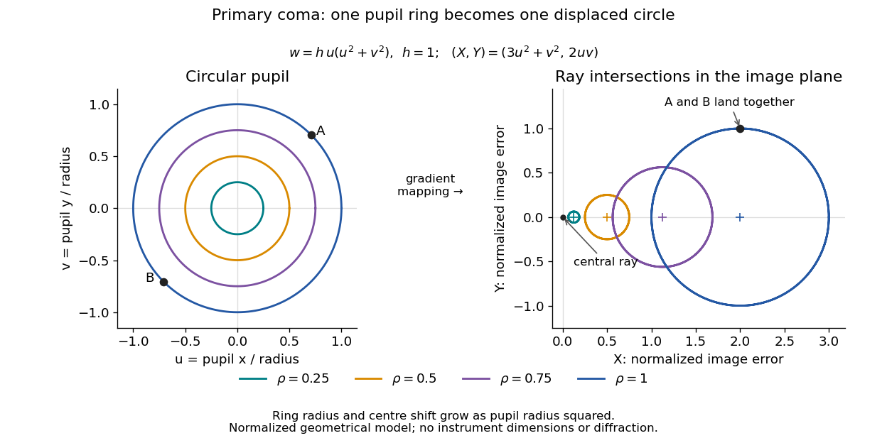
Consider an original, explicitly normalized model of primary coma, rather than a prescription for a particular optical lens. Let $(u,v)$ be Cartesian coordinates in a circular optical pupil divided by its radius $a$, with $u^2+v^2\le 1$. Let $h=\alpha /{\alpha }_0$ be a signed small field angle divided by an arbitrary positive reference angle. With polar coordinates $u=\rho \cos \theta$, $v=\rho \sin \theta$, prescribe the wavefront errorHere $W_0$ is an arbitrary positive optical path difference scale, not a measured error. The cubic optical pupil dependence and linear field dependence are the classical Seidel form.^[ref]

In the paraxial approximation, light ray direction errors follow the transverse gradient of wavefront error. For a reference sphere a distance $L$ from the exit optical pupil in a uniform image medium of refractive index $n$, the corresponding image-error scale is $s=L{W}_0/(na)$. Choose image-error coordinate signs so the normalized displacement is $\nabla w$; reversing the convention reverses the plotted orientation. Image coordinates below are errors relative to the ideal image of this particular object point, rather than positions of different objects:The partial derivatives explain the asymmetry: opposite optical pupil points $(u,v)$ and $(-u,-v)$ land together, rather than on opposite sides of the ideal image. For $h>0$, every $X$ is nonnegative, while $Y$ can have either sign. The figures stipulate this single wavefront error, omit other optical aberrations and diffraction, and assign no instrument dimensions.

For a ring of fixed optical pupil radius $\rho$, the double-angle formulas for trigonometric functions giveThus each ring maps into a circle of radius $|h|{\rho }^2$ whose centre is displaced by $2h{\rho }^2$. Doubling $\rho$ quadruples both sizes; for $h=1$, the edge ring has centre $(2,0)$ and radius $1$, while the half-radius ring has centre $(1/2,0)$ and radius $1/4$. Superposing these displaced circles produces the comet-like envelope.

For uniform irradiance over the circular optical pupil, equal area samples give an equal-weight geometrical image. Its centroid is $(h,0)$ because $⟨u^2⟩=⟨v^2⟩=1/4$ and $⟨uv⟩=0$. Moving the coordinate origin to that centroid translates the image; it does not remove its asymmetric shape. Adding a linear term to $w$ likewise translates all light rays equally. These origin choices must be distinguished from changing the optical aberration itself.

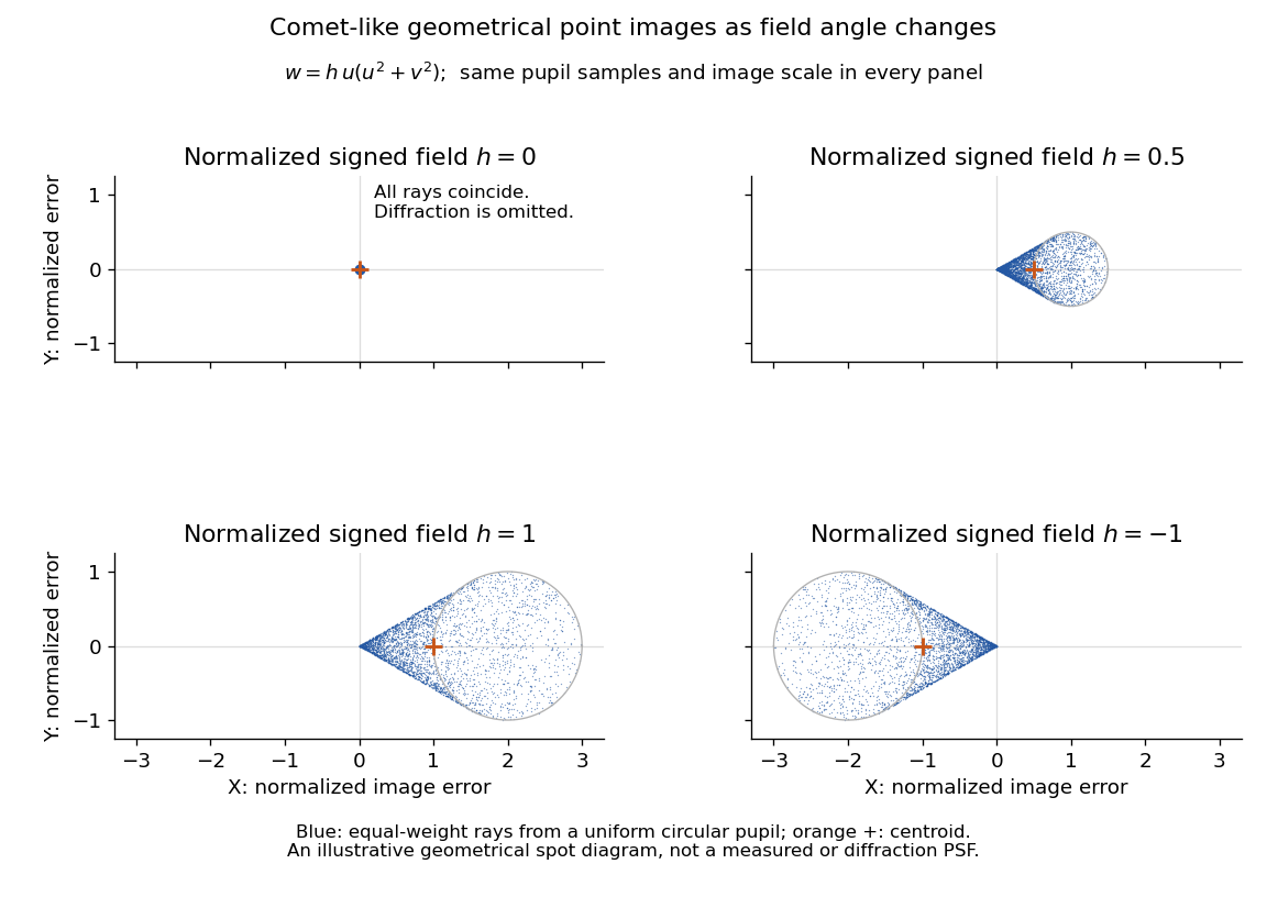
The model's full transverse extent is $3|h|$ along $X$ and $2|h|$ along $Y$. Halving the field angle halves the blur, and reversing it reverses the pattern about the ideal image. This isolates why coma matters for an optical camera's usable field of view: collecting more light does not ensure that off-axis points remain compact. Near diffraction-limited resolution, a physical optics calculation of the point spread function is needed instead of interpreting the geometrical tip as an infinitely sharp image.^[ref]

A semicircular disk is one half of a disk cut along a diameter, including its interior. It is a circular sector of angle $\pi$, with area $\pi a^2/2$. Source polar coordinates use $0\le r\le a$, $0\le \theta \le \pi$, and area element $rdrd\theta$. Its boundary consists of a semicircle and a diameter; the semicircle alone is a curve and has no planar interior.

The distance from a focus to a conic section along a line perpendicular to its symmetry axis. In focus-centred polar coordinates, an ellipse may be written $r(1-e\cos \theta )=\ell$, where $e$ is its eccentricity of a conic.

The distance from a focus of a conic section to the curve measured perpendicular to its principal axis. In the focus-based polar coordinates equation $r=p/(1+e\cos \varphi )$ it is the length $p$, where $e$ is the eccentricity. For an ellipse, $p=a(1-e^2)=b^2/a$. For a Newtonian Kepler orbit, $p=j^2/(GM)$ with $j$ the specific angular momentum.

For angular Fourier modes of integer order $n\ge 2$, the biharmonic equation in polar coordinates has radial basis $r^n,r^{-n},r^{n+2},r^{2-n}$. Apply the Laplacian twice to obtain the displayed indicial equation. For $n=0$, repeated roots give the radial basis $1,\log r,r^2,r^2\log r$; for $n=1$, the basis is $r^{-1},r,r\log r,r^3$. These are Cauchy-Euler equations. Regularity at the origin and boundary conditions select the admissible powers. For $n=2$, a constant radial factor still multiplies $\cos 2\theta$ or $\sin 2\theta$, so it is bounded but fails continuity at the origin.

For a counterclockwise, piecewise smooth simple closed planar curve $C$ enclosing $D$, Green's theorem with $P=-y/2$ and $Q=x/2$ gives $\frac{1}{2}{\oint }_C(xdy-ydx)={\iint }_{D}1dxdy$. The integral is the area of $D$ with a sign determined by the traversal direction. For polar coordinates $x=r\cos \theta$, $y=r\sin \theta$, differentiation gives $xdy-ydx=r^{2}d\theta$, yielding the familiar polar area formula when the curve is traversed once.

An ordinary scalar wavefunction assigns one complex amplitude to each physical configuration. In polar coordinates without an additional twisted boundary condition, the points $(r,\varphi )$ and $(r,\varphi +2\pi )$ are identical, so the angular factor must be periodic. An angular eigenfunction $e^{im\varphi }$ therefore requires integer $m$. This scalar orbital condition does not rule out half-integer intrinsic spin.

Consider a flat circular disk of radius $a>0$, with its center a perpendicular distance $d>0$ from the viewpoint $O$. The line from $O$ to its center is normal to the disk. Its rim defines a right circular cone with $\tan \theta =a/d$ and $\cos \theta =d/\sqrt{d^2+a^2}$. The solid angle of a circular cone immediately givesFor $a=d$, this is the same $45^{\circ }$ half-opening example: about $1.8403$ steradians. Both the radius and distance enter; doubling both leaves the solid angle unchanged.

A useful local version applies to a small surface patch of area $dA$, at distance $r$ from $O$. If $\psi$ is the angle between its unit normal and the line to $O$, its unsigned geometric contribution isThe numerator is the projected area. For a visible patch, perpendicular projection followed by radial projection onto a small piece of a sphere gives this formula. Integrating counts the directions once provided no direction encounters multiple counted patches. For an opaque detector, use its unoccluded face. At grazing view, the projected area tends to zero.

For this on-axis disk, a ring of radius $\rho$ has $r=\sqrt{d^2+{\rho }^2}$ and $|\cos \psi |=d/r$. Its polar coordinates gives $dA=\rho d\rho d\varphi$, so the same answer follows directly from the surface integral:The changing distance and obliquity are both already accounted for; an extra detector-wide cosine factor would count the projection twice.

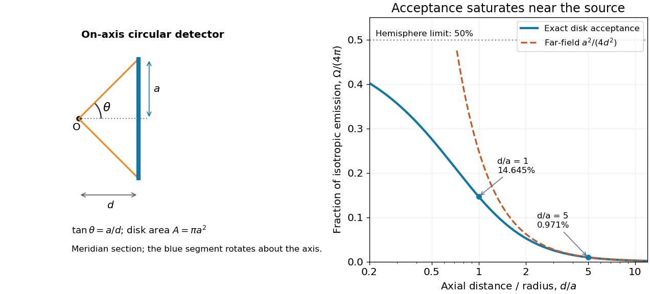
For $d\gg a$, the Taylor series of $(1+a^2/d^2{)}^{-1/2}$ givesThus the accepted fraction of an ideal point emitter's isotropic output is approximately $A/(4\pi d^2)$, where $A=\pi a^2$. This is the geometry behind the inverse-square law for a small detector. At fixed $a$, however, taking $d\to 0^{+}$ gives $\Omega \to 2\pi$, so the accepted fraction approaches $1/2$ rather than diverging.

For a chosen numerical example, let $a=1\mathrm{cm}$ and $d=5\mathrm{cm}$. The exact solid angle is approximately $0.122015$ steradians, giving an acceptance fraction $0.00970966$. An ideal point emitter with isotropy and total radiant flux $1\mathrm{mW}$ would therefore send about $9.71\mu \mathrm{W}$ onto the disk. The distant-source approximation gives $10.0\mu \mathrm{W}$, about $3.0\%$ high. This calculation assumes unobstructed propagation and counts incident radiant flux; photon absorption, detector response, and any optical attenuator require separate factors.

For motion confined to a plane but retaining potential energy $-\kappa /r$, separation in polar coordinates gives angular wavefunctions $e^{im\varphi }$ with integer $m$. The regular radial factor behaves as $r^{|m|}$ at the origin. Removing this power and the decaying exponential function leaves an Generalized Laguerre polynomial differential equation. polynomial termination requires $N=n_r+|m|+1/2$, yielding the displayed energy. At fixed $q=n_r+|m|$, the spinless quantum degeneracy is $2q+1$. This is not the logarithmic potential of electrostatics formulated entirely in two spatial dimensions.

Consider the original two-electron example obtained by taking $N=2$ in the Laughlin wavefunction, with no additional polynomial for the centre of mass. Introduce $Z=(z_1+z_2)/2$, relative complex coordinate $w=z_1-z_2$, separation $r=|w|$, and dimensionless separation $u=r/{\ell }_B$. Since $|z_1{|}^2+|z_2{|}^2=2|Z{|}^2+|w{|}^2/2$, the probability density factorizes:Integrating out $Z$ leaves an isotropic relative probability density. Define $D_m(u)$ per unit dimensionless area and $p_m(u)$ per unit dimensionless separation:The physical areal probability density is $D_m(r/{\ell }_B)/{\ell }_B^2$. The probability of a separation between $r$ and $r+dr$ is $p_m(r/{\ell }_B)dr/{\ell }_B$. The extra $u$ comes from the Jacobian determinant in polar coordinates: a thin annulus has area $2\pi rdr$. Omitting that factor changes the question being answered.

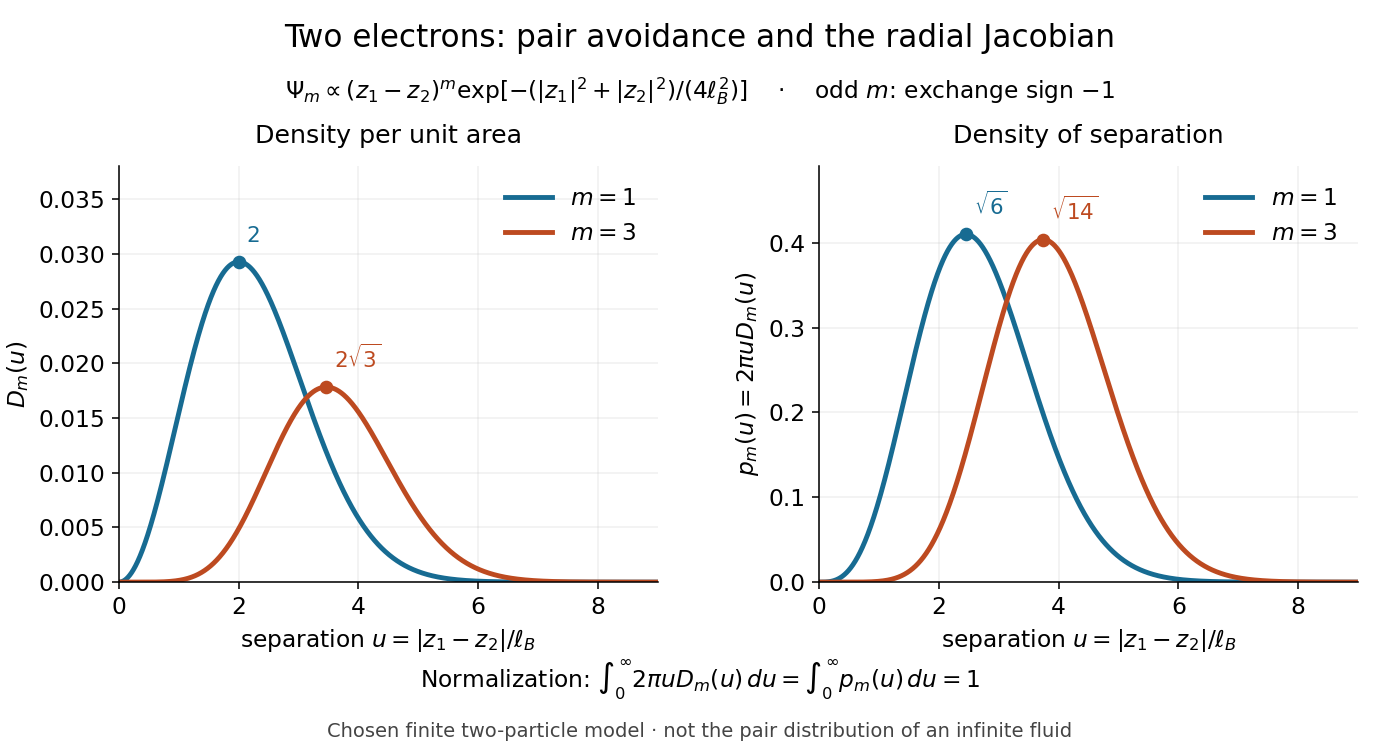
Both wavefunction normalization and the peak shift can be checked exactly. The substitution $t=u^2/4$ gives the Gamma function integralFor $m>0$, logarithmic differentiation givesConsequently the areal maximum lies at $u=2\sqrt{m}$, while the most probable separation lies farther out, at $u=\sqrt{4m+2}$. For $m=1$ these are $2$ and $\sqrt{6}\simeq 2.449$; for $m=3$, $\sqrt{12}\simeq 3.464$ and $\sqrt{14}\simeq 3.742$. The same substitution gives $⟨u^2⟩=4(m+1)$, so the root mean square separations are $\sqrt{8}$ and $4$ respectively. The distinction between a probability density maximum and a radial maximum therefore has a directly calculable geometric origin.

This two-electron model explains exchange and pair avoidance. It does not establish a nonzero many-particle spectral gap, an extended quantum Hall plateau, or the topological properties of a fluid in the thermodynamic limit. Those require additional many-electron reasoning and experimental tests.

The planar system $\dot{x}=y+(1-x^2-y^2)x$, $\dot{y}=-x+(1-x^2-y^2)y$ has polar coordinates $\dot{r}=r(1-r^2)$, $\dot{\theta }=-1$. Every nonzero orbit approaches the clockwise unit-circle limit cycle, of period $2\pi$. For $r(t_0)=r_0>0$,Interior orbits approach the origin backward in time, but exterior orbits have backward finite-time blow-up of an ordinary differential equation at $t=t_0+\frac{1}{2}\log (1-r_0^{-2})$. Thus forward convergence to a limit cycle does not imply existence for all negative times.

Use a velocity potential to reconstruct an irrotational flow from one scalar field. A velocity potential $\varphi (\mathbf{x},t)$ satisfiesIt has units ${\mathrm{m}}^2{\mathrm{s}}^{-1}$ and is unchanged as a description of the velocity field when any function of time alone is added. For twice continuously differentiable $\varphi$, the identity curl of a gradient proves zero vorticity. In incompressible flow, taking the divergence also gives ${\nabla }^2\varphi =0$, the Laplace equation. This turns a three-component velocity field into a single harmonic function with appropriate boundary conditions. ^[ref]

For uniform flow $\mathbf{u}=(U,0,0)$, take $\varphi =Ux$. With $U=2\mathrm{m}{\mathrm{s}}^{-1}$, the change from $x=0$ to $x=3\mathrm{m}$ is $\Delta \varphi =6{\mathrm{m}}^2{\mathrm{s}}^{-1}$. By the fundamental theorem for line integrals, the line integral of velocity between these points equals that change along any path in the domain; a closed curve gives zero circulation.

For the potential line vortex, choose a local angle branch in polar coordinates and set $\varphi =K\theta$. Then $u_r={\partial }_r\varphi =0$ and $u_{\theta }=r^{-1}{\partial }_{\theta }\varphi =K/r$. One counterclockwise turn changes the continued velocity potential by $2\pi K$, although the velocity field returns to its original value. With $K=1{\mathrm{m}}^2{\mathrm{s}}^{-1}$, this change is $2\pi {\mathrm{m}}^2{\mathrm{s}}^{-1}$, exactly the circulation. A full annulus therefore admits local angle branches and a multivalued velocity potential, but no global single-valued velocity potential when $K\ne 0$. Cutting the annulus along a radial line allows a single-valued angle branch on the remaining domain. The obstruction is path independence, not a failure of the local gradient formula.

At $q=a=(r-1)/(r+1)>0$, the reaction eigenvalues are $\pm i\sqrt{a}$. This linear marginal case is a weakly attracting focus, not a nonlinear center. To check it directly, put $u=(1+r)(1+x)$, $v=(1+r{)}^2(1+y)$, $h=(1+a)/2$, $\beta =(1-a)/2$, $\omega =\sqrt{a}$, and $X=x$, $Y=(hy-ax)/\omega$. The equations become $\dot{X}=-\omega Y+F_2+F_3+O(4)$, $\dot{Y}=\omega X+G_2+G_3+O(4)$, withOn the unit circle write $A=\cos \theta F_2+\sin \theta G_2$, $B=\cos \theta F_3+\sin \theta G_3$, $C=\cos \theta G_2-\sin \theta F_2$. In polar coordinates, $d\varrho /d\theta =(A/\omega ){\varrho }^2+(B/\omega -AC/{\omega }^2){\varrho }^3+O({\varrho }^4)$. The quadratic angular average vanishes. Integrating the quadratic correction over a whole cycle contributes its final squared integral, also zero, leaving the cubic average. Using the even trigonometric moments gives $⟨B⟩=a/4$ and $⟨AC⟩/\omega =(a+1)/8$. The Poincaré map is therefore $\varrho \mapsto \varrho +[2\pi /\omega ](a-1){\varrho }^3/8+O({\varrho }^4)$. Since $0<a<1$, it contracts sufficiently small positive radii and proves nonlinear asymptotic stability at the threshold.