The expectation value of a quantum observable is the expected value of its measurement outcome random variable in a specified quantum state. It predicts the mean of outcomes from many identical quantum state preparations. It need not equal any one possible outcome: for a spin one-half particle, equal probabilities of and give mean zero even though zero is never an outcome of that spin component. Here is the reduced Planck constant.
Let be a Hermitian operator on a finite-dimensional Hilbert space, and let be a normalized pure state, . The spectral theorem writesThe are distinct real eigenvalues, are orthogonal projections onto their eigenspaces, and is the identity operator. For an ideal projective measurement of , the Born rule and the expectation value giveThus the expectation value is a probability-weighted average of eigenvalues, including all vectors in a degenerate eigenspace in its . In an orthonormal eigenbasis, , this is , where repeated are allowed. The weighted average lies between the smallest and largest eigenvalues; it can lie in a gap between them. The statistical meaning and operator expression are connected in this way in the authored treatment of average energies.[ref]
Chapter 20: Operators. The Feynman Lectures on Physics, Volume III, Chapter 20: Operators, §20–2, equations (20.11)–(20.20): outcome frequencies, weighted mean, and operator expectation
If a nonzero vector has not been normalized, use ; the denominator is essential. A global phase cancels between the bra and ket, so and have the same expectation value and outcome probabilities.
The outcome variance measures the spread about this mean, whereas the quantum uncertainty is its standard deviation:For a pure state, zero variance means that lies entirely in one eigenspace. That eigenspace need not be one-dimensional. Knowing only a mean generally does not determine the entire outcome probability distribution.
For a mixed state, the same formulas use its density matrix , a positive operator with trace one:A pure state is the special case . For a quantum state ensemble , the expectation value is . This linearity is useful when preparations vary between trials; different quantum state ensembles can have the same density matrix.
These formulas require no operator-domain qualifications in finite dimension. For an unbounded self-adjoint operator, the spectral theorem instead gives a spectral probability measure; a finite mean requires an integrable absolute first moment, and finite variance requires a finite second moment. Writing as an operator inner product additionally requires in the operator domain of . The quadratic form of a positive quantum Hamiltonian explains the useful wider form-domain version.
For spin one-half, choose the normalized spin eigenstates with . The spin one-half along an axis pure state in the plane isIts norm is one because the two eigenstates are orthogonal and . Applying the Born rule to a projective measurement givesConsequently the expectation value, second moment, and variance areAt , the outcome probabilities are and , the mean is , and the variance is . Every individual outcome remains . At , the mean is zero and the variance is maximal, . At either pole, one outcome has probability one and the variance vanishes.
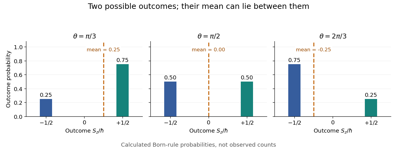
Spin expectation value between the two possible outcomes
. Original calculated Born rule distributions at three preparation angles. Bar heights are outcome probabilities; the dashed orange line marks the expectation value, whose horizontal position is usually not an allowed outcome. Spin values are expressed in units of the reduced Planck constant. No bars represent experimental observations. Source. Details.The diagonal mixed state has the same probabilities, expectation value, and variance as . It is nevertheless a different quantum state for : the displayed pure state has , while has . A single component's mean does not reveal all relative quantum phases or establish purity of a density operator.
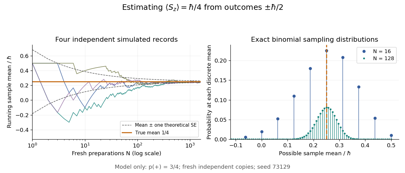
Prepare a fresh copy of the same quantum state for each trial and measure the same observable. If preparations and readouts are independent, the outcomes are independent and identically distributed random variables with the Born rule probability distribution. Their sample mean is an unbiased estimator of the expectation value:The law of large numbers explains convergence of the sample mean, while the standard error describes its finite-sample spread. It takes four times as many independent trials to halve that standard error. This reduces estimation error; it does not reduce the quantum uncertainty of a single prepared copy.
For the spin expectation value, let and be the two outcome counts, with . ThenThe binomial distribution gives the exact sampling model. For , the standard error is : approximately for and for . A run can fluctuate away from the predicted mean even as its typical spread decreases.
Repeatedly measuring one surviving system is a different protocol. Under the ideal Lüders rule, outcome leaves when . With no intervening change of observable or dynamics moving the state out of that eigenspace, the next projective measurement returns with certainty. Such a record is correlated and does not sample the original Born rule distribution independently. The quantum nondemolition measurement discussion describes this repeatability; fresh quantum state preparations supply the ensemble needed for the estimator above.
A concrete idealized implementation uses a Stern-Gerlach experiment twice: a preparation filter along passes only its plus spin channel, and a analyzer resolves both output channels for many fresh atoms. This prepares the spin one-half along an axis state . The authored apparatus description uses slit collimation, a nonuniform magnetic field with a pointed pole, and counters at the separated outputs.[ref]
Chapter 5: Spin One. The Feynman Lectures on Physics, Volume III, Chapter 5: Spin One, §5–1, figure 5–1 and the paragraph proposing output counters; §5–4, slit diffraction and internal-state limitations
The two-channel spin one-half preparation and analyzer are described separately; the source's recombining “improved” apparatus is explicitly idealized, so the setup here is a proposed estimation model, not a report of observed counts.[ref]Count every accepted analyzer event in its calibrated or channel and compute from the count difference. The magnetic field gradient separates trajectories through their magnetic moments; calibrated channel labels convert positions into spin eigenvalues. The readout is a population imbalance, not an intermediate trajectory carrying spin . Beam position also depends on flight time and field geometry, so averaging raw positions alone does not establish a calibrated spin expectation value.
As controls, feed known and preparations to check the channel assignment and leakage, hold the analyzer axis fixed, and repeat short blocks to check preparation drift. Measure background counts and relative channel efficiencies. With efficiencies and and negligible background, the detected plus fraction isUnequal efficiencies bias the naive sample mean, even for arbitrarily many counts. For example, , , and give detected fraction and naive mean , rather than . Background, overlapping beams, detector saturation, angle misalignment, unwanted internal states, and preparation correlations require a better measurement in quantum mechanics model. Increasing only reduces the independent sampling contribution; it cannot remove these systematic errors. The selected preparation beam is the population being estimated, so losses in preparing it must be distinguished from losses in reading its two outcomes.