The foundations of quantum mechanics study the physical and conceptual status of quantum states, measurement, nonlocal correlations, and possible extensions of quantum theory.
A theory is complete in the EPR sense only if its description represents every element of physical reality. Their sufficient reality criterion uses certain prediction without disturbance. Applying it to alternative measurements on a remote partner also requires an independence premise concerning the unmeasured system's physical reality; that premise must not be suppressed when presenting the argument.[ref]
Can Quantum-Mechanical Description of Physical Reality Be Considered Complete? by Albert Einstein and others. 1935, pages 777 and 779–780
The need for mutually exclusive experimental arrangements or incompatible observables to exhibit different aspects of a quantum system. For example, path discrimination and interference contrast obey a tradeoff, while sharp Pauli operator and measurements have incompatible eigenbases. Which-path information is an operational record, rather than a requirement that a conscious observer reads it.
An interpretation retaining universal unitary evolution of the quantum state, with definite measurement records described relative to outcome branches. Quantum decoherence explains the practical isolation and stable record basis of emergent branches. It does not insert a physical collapse selecting just one component. The emergence of branch structure and justification of Born rule weights involve additional interpretive arguments beyond writing the Schrödinger equation.
Uncertainty about which observer-centred situation is one's own, even conditional on a known global wave function. An example is a post-measurement observer who has not yet consulted a decohered record. This proposal distinguishes uncertainty about the experienced record from randomness in the universal dynamics. A further argument is needed to connect its credences to branch weights; not every decision-theoretic Everettian account must interpret its weights as ignorance of a uniquely selected future branch.
For an orthogonal decomposition , the squared norms add to the total norm. Refining one component into orthogonal subcomponents preserves its total weight by the Pythagorean theorem. In an Everettian account these weights are candidates for governing probabilities, rational credences or decisions; the algebra alone does not select which interpretive role is justified. Counting arbitrarily refined components is not the same measure.[ref]
An approach assigning probabilities to compatible families of time-ordered quantum alternatives. A decoherence functional measures interference between histories; when its relevant cross-terms vanish, coarse-grained probabilities add as in probability theory. Different incompatible families must not be combined as if they were one classical history space. The formalism does not require a fundamental external measurement apparatus.
For alternatives represented by projection operators at successive times, set in the Heisenberg picture. The displayed functional uses the initial density operator . Combining two histories gives . Thus vanishing real cross-terms gives the probability sum rule; the stronger commonly used condition for distinct histories is sufficient as well. Its diagonal is nonnegative because each is positive.
The EPR argument uses correlations of an entangled state and a locality assumption to challenge the completeness of the quantum description. Its Einstein–Podolsky–Rosen criterion of reality identifies quantities predictable with certainty without disturbing a distant system as elements of physical reality.
For a shared quantum entanglement resource, one party's choice of measurement can prepare different conditional ensembles for the distant party. Discarding the outcome leaves the same distant reduced density matrix, so steering does not itself permit signalling. Demonstrating steering against a local hidden-state model is stronger than merely observing a change in a postselected description.
For a Bell pair , Alice's basic measurement in the entrywise complex conjugate of any desired Bob orthonormal basis prepares each Bob pure state with probability . Indeed, if , then , which proves the displayed contraction identity. The undisclosed-outcome density matrix stays ; quantum steering changes the conditional quantum state ensemble without violating the no-communication theorem.
The Einstein–Podolsky–Rosen criterion says that if one can predict a physical quantity with certainty without disturbing the system, then there is an element of physical reality corresponding to that quantity.
A superselection rule partitions a representation into sectors between which the specified observable algebra has no matrix elements. Relative phases between vectors in different sectors cannot be detected by those observables, so a coherent vector spanning sectors and its sector-diagonal mixture define the same observable state. The restriction is relative to the observable algebra; it is not by itself a physical wave-function collapse. Infinite-system phases can yield disjoint representations and emergent superselection sectors even though each finite system permits global connecting operators.
The certainty of a prediction made without disturbing the system is proposed as sufficient evidence that the predicted quantity corresponds to an element of physical reality. It motivates the discussion of completeness and locality in foundations of quantum mechanics, but is distinct from the conditional factorization assumed by local hidden-variable theory.
A deterministic interpretation with a definite particle configuration guided by the wavefunction. The latter obeys the Time-dependent Schrödinger equation, while the particle follows the guidance equation. A Born rule distribution of initial positions is preserved by quantum equilibrium equivariance. The guidance law restricts admissible initial velocities, even when trajectories are rewritten as a second-order force equation.
The ensemble density of actual configurations equals the squared norm of the guiding wave function. For spinless particles with , the Schrödinger continuity equation is . A density transported by the same guiding field satisfies the same equation, so initial equality is preserved. This equivariance is a consistency property, not a proof that every possible initial ensemble is in equilibrium. The physical account of the equilibrium assumption and subsystem statistics requires an additional argument.
In the spinless version of Bohmian mechanics, insert the actual environment configuration into a total wave function to obtain a subsystem's conditional wave function, when that slice is nonzero. It encodes the actual environment relevant to the subsystem's guiding dynamics. It need not satisfy an autonomous subsystem Schrödinger equation; further separation conditions are needed for an effective wave function.[ref]
If total-wave branches become disjoint in the relevant environment configuration variables and the actual environment lies within one branch, the subsystem's conditional wave function is proportional to that branch's subsystem factor. Persistent separation makes its autonomous use an effective description. No term of the universal wave function has literally been deleted. Possible recombination prevents treating every temporary packet separation as irreversible collapse.[ref]
An interpretation treating the universal wave function as part of the law governing actual configurations rather than an additional material field. The interpretation is motivated partly by the absence of reciprocal configuration-to-wave influence in Bohmian mechanics.[ref]
Bohmian Mechanics and the Meaning of the Wave Function by Detlef Dürr and others. discussion of the universal wave function as law-like
If and the actual environmental configuration lies in the support of disjoint from the environmental support of , then evaluating the guidance equation at gives the velocity generated by . This is effective collapse without deleting a universal empty wave.
A component of the wave function whose configuration-space support does not contain the actual configuration. It can affect later guidance equation evolution if branches overlap again; enduring environmental separation makes it dynamically irrelevant to the occupied branch to excellent approximation.
For the separation of a two-dimensional central-potential eigenstate, the guidance equation gives zero radial velocity and constant-radius circular motion, with circulation . A real superposition of the degenerate and eigenstates has zero current away from nodes instead. The speed depends on the actual wavefunction, not just its energy.
The amplitude-dependent extra potential in the Madelung equations. Taking the gradient of their phase equation and using the guidance equation yields , where is the material derivative. At wavefunction nodes this local expression may be singular.
For a spinless particle without a magnetic vector potential, Bohmian mechanics sets , where is the dimensionless quantum phase. Equivalently the velocity is the probability current divided by the probability density. This formula is local to nonzero wavefunction regions.
Both the ensemble position density transported by the guidance equation and the squared wave amplitude satisfy the same probability continuity equation. Subject to existence and uniqueness of that transport, an initial Born rule distribution stays a Born rule distribution. This is a preservation statement, not a derivation that every initial ensemble is already in equilibrium.
An ontological model associates each quantum state preparation with a probability distribution over underlying physical states . A measurement in quantum mechanics's response probabilities depend on its specification and , sum to one, and reproduce the Born rule when averaged over the preparation distribution. The model need not assign deterministic outcomes. Overlap or disjointness of preparation measures defines the psi-epistemic model versus psi-ontic model distinction.
Under preparation independence, an ontological model of a quantum system reproducing exact quantum quantum measurement probabilities cannot assign overlapping preparation measures to distinct pure states. An exclusion quantum measurement on independent copies makes every outcome impossible for one possible preparation; a common ontic region would require every response to vanish there. Thus the conclusion is a psi-ontic model, not a blanket exclusion of hidden variables or all informational interpretations.
If two pure quantum states overlap by , their -copy states have overlap . Each block spans an effective qubit, with orthonormal basis and . Applying the two-block PBR exclusion measurement for zero and plus uses independently prepared copies. A common single-copy ontic overlap of positive mass remains positive under this finite tensor power.
The product preparations are excluded respectively by the orthonormal vectors , , and , written in the computational basis. Each vector has zero inner product with its labelled preparation. This projective measurement gives antidistinguishable quantum states and drives the two-copy PBR theorem contradiction.
Independently operated quantum state preparations are assumed to produce independent underlying physical states. Their joint preparation measure factors into the single-system measures. This ontic factorization is an additional assumption, not a consequence of operational independence alone. It turns a common single-system overlap of mass into a common -system overlap of mass in the PBR theorem.
An ontological model of a quantum system is psi-epistemic if some pair of distinct pure states has preparation measures with nonzero overlap. The same physical state can then be compatible with either preparation. This precise measure-overlap definition is stronger than merely interpreting a wave function as information or a computational tool.
An ontological model of a quantum system is psi-ontic if distinct pure states have mutually singular preparation distributions. The physical state then determines which pure quantum state was prepared, almost surely in the pairwise sense. Extra underlying variables may still exist. The PBR theorem establishes this conclusion under preparation independence and exact quantum predictions.
Bell's theorem shows that no theory assigning outcomes through local hidden variables can reproduce every quantum correlation.
The force of the Bell theorem is that a disagreement about a local hidden-variable theory becomes a constraint on frequencies in a Bell test. Quantum entanglement alone does not guarantee a violation for every measurement in quantum mechanics: the quantum state, analyzer settings and treatment of missed events all matter. A violation of the CHSH inequality tests the conjunction of Bell local causality, measurement independence and the stated outcome and sampling assumptions; it remains compatible with quantum no-signalling.
Quantum correlations incompatible with Bell local causality under additional assumptions including measurement independence. This is an operational statement about joint probabilities, not controllable faster-than-light signaling: quantum predictions also obey quantum no-signalling. Entanglement alone does not guarantee violation of a specified Bell inequality in a given measurement arrangement.
A two-setting nonlocality argument in which several zero-probability events forbid a further coincidence in any deterministic local hidden-variable model, but quantum theory assigns that coincidence positive probability. For binary indicators, suppose , and . Any assignment with would violate the first relation. A quantum implementation can nevertheless give such a coincidence. Real imperfect experiments require an inequality that accounts for their nonzero error probabilities. Lucien Hardy gave a two-particle inequality-free argument in 1992.[ref]
A Bell test compares experimental probabilities or expectation values with a Bell inequality. In a two-setting photon polarization test, each station chooses a polarizer orientation and records an outcome. A coincidence circuit identifies candidate pairs using an agreed timing rule. The choice of which trials enter the statistic is part of the experiment: correlations calculated only from detected pairs can differ from correlations of all emitted pairs. The Polarization CHSH count model separates ideal expectation values from this experimental selection problem.
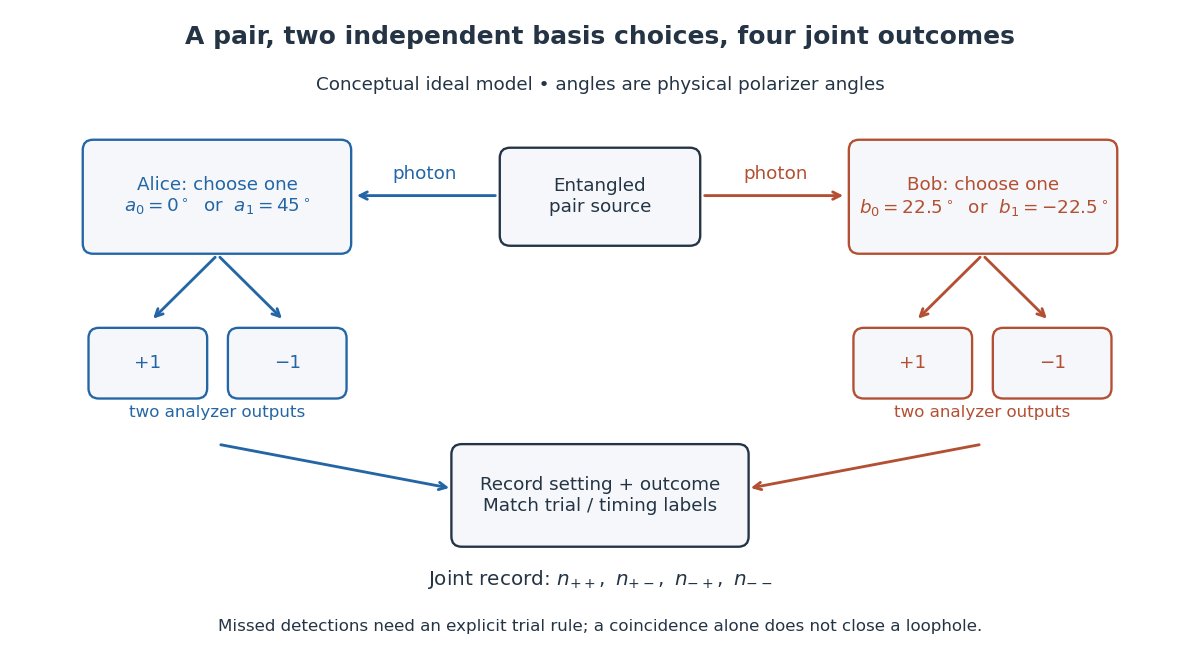
Two-setting polarization measurements and coincidence readout
. Conceptual apparatus for the ideal two-output model. The displayed angles belong to the worked CHSH example; they are not a reconstruction of a historical apparatus. Each station chooses one basis, then records either output. The coincidence record also needs a rule for missed detections. Details.
The Bell test reported by Bas Hensen and collaborators used electron spins separated by , efficient spin readout and rapid random measurement settings. Those features addressed detection and locality loopholes together. Its result tests Bell local causality with the stated experimental assumptions, rather than ruling out every possible hidden-variable theory.[ref]
Experimental loophole-free violation of a Bell inequality by Bas Hensen and others. 2015 abstract: spin separation, efficient readout and basis-choice timing
In 1972, Stuart J. Freedman and John F. Clauser excited a calcium beam from an oven with a filtered deuterium arc lamp. A calcium emission cascade supplied paired photons; an optical lens system, optical filters, removable glass-plate polarizers and cooled photomultipliers selected their linear polarizations. They compared coincidence circuit rates at relative angles and , normalized with polarizers removed. Alternating configurations controlled drift; delayed counts estimated accidental coincidences. The violation agreed with quantum mechanics, conditional on their explicit assumption that passage through a polarizer did not change a photon's detection probability. This was a static-analyzer test with a detection loophole, rather than the ideal four-output CHSH inequality statistic.[ref]
In 1982, Alain Aspect, Jean Dalibard and Gérard Roger used a calcium cascade and an acoustic standing wave in water to route each photon toward one of two fixed polarizers. Switching took about , against for light to cross between stations. Photomultiplier coincidence circuit rates, with delayed-background subtraction and polarizer-removal normalization, violated their Bell inequality. Supplementary polarizers checked each channel against Malus's law. The timing attacked the locality loophole, but the authors emphasized that switching was quasiperiodic, not random; incomplete switching and inefficient collection also limited the test. Its normalized statistic differs from the CHSH inequality convention used below.[ref]
Experimental Test of Bell's Inequalities Using Time-Varying Analyzers by Alain Aspect and others. pp. 1805-1807, Figs. 2-4; final discussion
In 1998, Jian-Wei Pan, Dik Bouwmeester, Harald Weinfurter and Anton Zeilinger created two photon pairs by two passages of a pulsed pump through a crystal using spontaneous parametric down-conversion. Interfering the inner photons at a nonpolarizing beam splitter implemented a partial Bell-basis measurement. Narrow optical filters and spatial filtering removed distinguishing information; changing the outer polarizer bases checked the conditional correlations. Fourfold detections selected the entanglement swapping events. The reported interference supported conditional quantum entanglement, but the paper reserved a statistically significant Bell inequality violation for improved visibility; it was not a demonstration closing the detection loophole.[ref]
Experimental Entanglement Swapping: Entangling Photons That Never Interacted by Jian-Wei Pan and others. pp. 3892-3894, Eq. (3), Figs. 2-3; visibility discussion
The ideal calculation makes the distinction between conditional and unconditional quantum states explicit. Start with spin singlet states , where and denote orthogonal photon polarizations. Taking the inner product with gives : expanding the four terms leaves precisely the two antisymmetric outer terms. That Bell-basis measurement outcome has probability and leaves the outer pair in a spin singlet state. Ignoring the inner outcome instead leaves the outer density matrix , a maximally mixed state. A conditional preparation flag is useful for later Bell tests only with the timing and setting conditions in setting-independent heralding preserves Bell locality.
In 2015, Marissa Giustina, Anton Zeilinger and collaborators combined spontaneous parametric down-conversion with rapid random analyzer choices and efficient transition-edge sensors. Local records included settings and detector signals; their Bell inequality used detected and undetected trials, avoiding fair sampling. Locally fixed time slots prevented coincidence-based trial selection. Calibrated optical and electrical delays checked spacelike separation of each choice from the remote readout. The violation addressed detection and locality together. Measurement independence still requires assumptions about the hidden state's origin; the experiment cannot exclude every possible common cause of source and settings.[ref]
The detection loophole arises when missed events allow the retained sample to depend on settings and hidden variables. For example, a local hidden-variable theory may retain different underlying pairs at different polarizer angles. Applying the CHSH inequality to that selected sample does not test the original setting-independent ensemble. A valid protocol specifies outcomes and trials, including failures, or justifies an appropriate fair sampling assumption. Subtracting accidental coincidences addresses background contamination; it does not by itself repair this selection problem.
For a specified Bell test statistic, fair sampling assumes that conditioning on successful detections preserves the correlations needed to represent the intended ensemble. Constant detector efficiency in an independently specified loss model can ensure this; constant observed count rates alone do not establish independence from the hidden state. The Polarization CHSH count model explicitly assumes independent losses.
The locality loophole permits a station's outcome to be influenced by the distant setting through an ordinary signal arriving before readout. Spacelike separation excludes such communication at or below the speed of light. Fast changes only help if the relevant choice and detection events have the required timing. Predictable switching also leaves open correlations with earlier settings; closing a communication channel does not prove measurement independence.
A Bell inequality is a constraint on observable correlations satisfied by the specified class of local hidden-variable models. In finite-setting scenarios such constraints bound linear combinations of probabilities or expectation values. The CHSH inequality is one example, following from Bell factorization, measurement independence and bounded outcomes. A violation rules out the conjunction of the assumptions defining that model class; it does not alone identify a unique false premise.
A bound on the correlations attainable by measurement in quantum measurements for a specified Bell expression. The CHSH Tsirelson bound is ; the number depends on which Bell expression is being optimized.
For dichotomic observables with , let . Expanding gives . Each commutator has operator norm at most two, so and . Appropriate spin measurements of a Bell state attain equality. The local hidden-variable bound of the corresponding CHSH inequality is two.
For outcomes in , let be their nonnegative modular representative. A deterministic local hidden-variable model satisfiesThe unreduced chain telescopes to , so its reduced nonnegative sum is at least for each assignment. For binary outcomes and two settings, it is a form of the CHSH inequality: .
On , measure , assigning bit to eigenvalue . Choose Alice's angles and Bob's angles , with . The Bell state correlation is . Each adjacent disagreement term and the last agreement term therefore has probability . For , their total violates the chained modular Bell inequality bound one, and it tends to zero as . At the value is exactly one.
// Target: probability-and-statistics.bigb
In a local hidden-variable description of a Bell experiment, shared hidden data have a distribution independent of the measurement settings. Each outcome depends on the local setting and those shared data, without dependence on the remote setting. Local randomness can be included in the hidden data. Perfect correlations then constrain simultaneous assignments to the possible local measurements. The GHZ theorem shows an all-versus-nothing inconsistency between such assignments and certain three-qubit correlations.
If a successful preparation flag is fixed before freely selected Bell inequality settings, conditioning a local hidden-variable theory on that flag only replaces its hidden-variable distribution by the conditional distribution. The later response functions remain local and the distribution is independent of the later settings, so the CHSH inequality still holds. Setting-dependent rejection during the Bell measurements does not satisfy this argument.
Outcome independence requires . It says that, once settings and the proposed complete state are fixed, learning the distant outcome does not change the local outcome probability. Combining it with parameter independence gives Bell factorization. Entangled quantum states generally fail outcome independence even though their observable marginal distributions obey quantum no-signalling.
For spacelike-separated measurement regions, a sufficient specification of their relevant past should screen each outcome from additional information in the other wing. In a two-setting experiment a Bell-local model has . Together with measurement independence and bounded outcomes, this implies the CHSH inequality. Bell local causality is stronger than quantum no-signalling and is not an assumption that every outcome was predetermined.
Outcome determinism says that a complete hidden state and the measurement settings fix each measurement outcome with probability one.
Parameter independence says that, conditional on the complete hidden state, the probability distribution of one party's outcome is independent of the other party's measurement setting.
Measurement independence says that the distribution of the hidden state is independent of the measurement settings: . Its failure is the measurement-dependence loophole in a Bell test.
A Bell-test loophole in which hidden information determining the device outputs is correlated with the chosen measurement settings. The usual local CHSH inequality averages a common hidden-variable distribution over independently selected settings. If that distribution can instead depend on the selected pair, the four counterfactual assignments need not obey the same averaging argument. An adversary controlling both the devices and their setting generators can exploit this dependence without violating the local-bound proof's actual hypotheses.
For local outcomes , the Clauser–Horne–Shimony–Holt inequality isAn arbitrary no-signalling correlation can reach the algebraic maximum , while quantum correlations are bounded by .
For a short proof of the local bound, fix a deterministic local hidden-variable model assignment. The combination is . Exactly one bracket vanishes and the other is , so every assignment contributes . Averaging with a single setting-independent probability distribution preserves the interval . Mixtures also cover stochastic local hidden-variable theories. Rejecting a different sample at each setting would invalidate precisely that common-average step.
The quantum bound follows just as economically. For Hermitian operators with , the CHSH inequality operator obeys . Each commutator has operator norm at most two, giving . The Polarization CHSH count model attains this bound without allowing either station to control the distant marginal probability distribution.
For the Bell state , let both zero-input measurements use the computational basis, and let the one-input bases be rotated by for Alice and for Bob in the real qubit plane. In the CHSH game, the four conditional winning probabilities are . They follow by contraction of the Bell state with vectors from the real orthonormal bases used for the basic measurements. Their average is the displayed expression. On , this beats exactly when and reaches at , since .
Two separated players receive uniformly random input bits and output bits without communicating after receiving their inputs. They win when , with exclusive or . For deterministic local response functions, the four desired equalities have inconsistent parity, so at most three can hold. Shared randomness only averages such strategies, proving classical winning probability at most . In terms of correlations , the winning probability is , directly connecting the game to the CHSH inequality.
The Hermitian operator has eigenvalues on , respectively. Thus any density matrix satisfying must be : an average can equal the largest eigenvalue only when all weight lies in its one-dimensional eigenspace. The purity decouples a subsystem from its purification lemma then excludes correlations with an external environment. This argument assumes the stated measurement operators; CHSH self-testing handles unknown representations with additional qualifications.
Maximal quantum CHSH inequality violation certifies an embedded maximally entangled qubit pair and its ideal measurement action, up to local isometries and unused ancillary systems, under the separated-device quantum assumptions. It does not identify every microscopic component of an arbitrary device. Near-maximal observed correlations require robust error bounds rather than exact identification.[ref]
Robust Self Testing of the Singlet by Matthew McKague and others. Robust Self Testing of the Singlet, arXiv:1203.2976, abstract: local bases isolate an approximate EPR pair, potentially encoded within a larger environment or ancilla
Let be orthogonal linear polarizations, and prepare the Bell state . The analyzer vector is ; its orthogonal companion has outcome . Direct inner products with the Bell state give and . Thus the expectation value of the outcome product is . These are physical polarizer angles; their corresponding Bloch sphere angles are doubled.
For a stipulated isotropic admixture, use the density matrixThe maximally mixed state contributes zero correlation, so for . Each local marginal is , independently of the other setting, illustrating quantum no-signalling. In this model is the interferometric visibility of the coincidence fringe; other noise models need not have one common visibility for every basis.
Choose , , and . The four correlations in the displayed CHSH inequality are . Consequently , exceeding the local bound exactly when . Perfect correlation at a single common setting would not yield this comparison between incompatible quantum measurements.
To connect probabilities with expected counts, stipulate emitted pairs per setting pair and independent detection efficiencies , independent also of settings, outcomes and hidden variables. The expected joint counts are . Their normalized correlation isFor original teaching inputs , , and , the expected counts are and . They total and give , hence . Fractional expected counts are not measured data. Efficiency cancels here because the loss model was specified to be independent; this algebra supplies no justification for discarding failures in an arbitrary Bell test with a detection loophole.
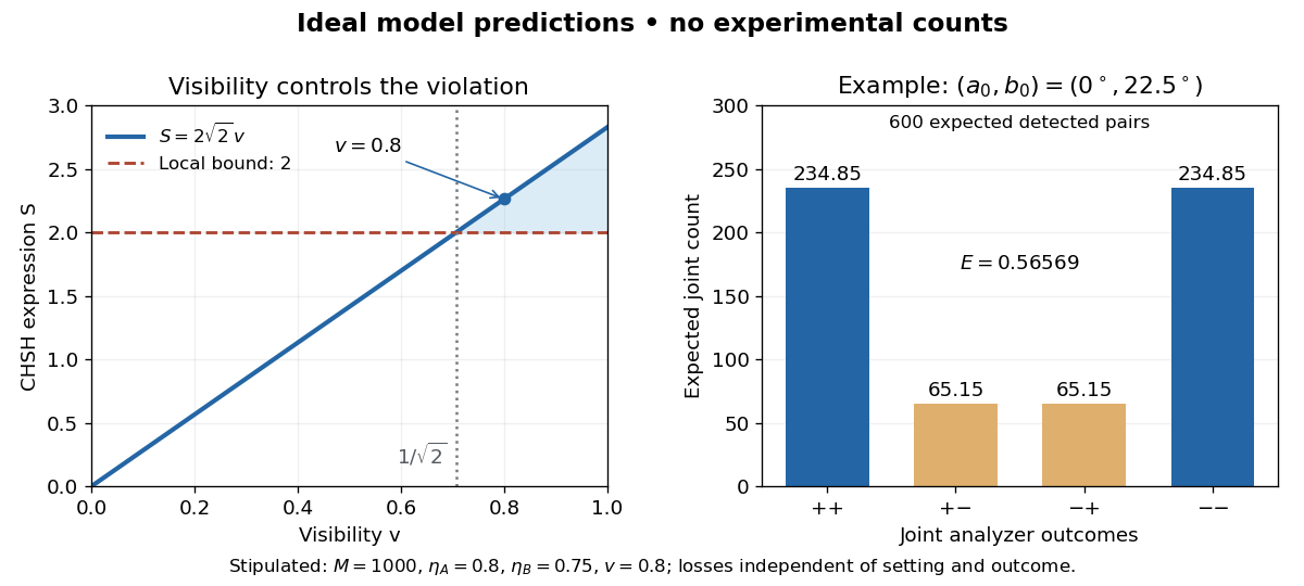
Ideal CHSH visibility threshold and expected detection counts
. Original model predictions, not experimental data. The first panel shows the visibility needed to exceed the local bound. The second uses 1000 emitted pairs, efficiencies 0.8 and 0.75, and visibility 0.8; each bar is an expected joint count. Details.
For spin-projective measurements on a two-qubit state, let be the eigenvalues of , where is its Pauli correlation tensor. Bob's sum and difference of unit axes are orthogonal and have lengths and . Maximizing Alice's two axes aligns them with the corresponding images under . Maximizing then gives for orthonormal . The maximum of this quadratic-form sum is , by diagonalizing and selecting its top two eigenvectors. Thus the displayed expression is both an upper bound and attainable. The same maximum applies to the form with the sum of two absolute values, since local outcome signs can select their positive branches.
Every entangled pure state of two qubits violates a CHSH inequality for a suitable choice of local measurement axes. If its two Schmidt coefficients are , the optimal construction already gives a value .
For the Schmidt-basis Pauli correlation tensor, choose Alice's axes and Bob's . The CHSH inequality expression is . It exceeds two exactly when both Schmidt coefficients are nonzero, reaching for maximal quantum entanglement. A product state gives and saturates rather than violates the inequality.
A no-signalling box is a conditional probability distribution whose marginal distribution for either party is independent of the other party's input. It can therefore exhibit correlations stronger than quantum correlations without transmitting information superluminally.
A Popescu–Rohrlich box is a bipartite no-signalling box attaining the algebraic maximum of the CHSH inequality.
Take a separated Boolean decomposition . Feed to one independent PR box, obtaining outputs with . Alice forms , Bob forms , and their parities satisfy . Sending the single bit lets Bob compute the answer with certainty. The truth-table decomposition needs at most boxes for input lengths . Each box's local output is uniform, so Bob's uncommunicated output string carries no information about Alice's input; the final parity bit is essential for a general function depending on that input.
An objective-collapse theory treats wave-function collapse as a physical process localized in spacetime, rather than only as an observer's update of information.
A Gaussian function used for localization is nonzero at every finite separation, so multiplying a wave function by it normally suppresses distant components without making them vanish. The interpretive question is how these residual, potentially structured components relate to definite macroscopic records. Exact compact localization and overwhelmingly concentrated matter are different claims.
The Ghirardi--Rimini--Weber theory modifies unitary time evolution by random Gaussian position localizations. Each constituent collapses at a small fixed rate, while the rate for an entangled macroscopic body grows with its number of constituents.
A version of the GRW model whose material events are collapse centres in spacetime. A macroscopic object is represented by a pattern of such events, not by particle trajectories between flashes. Exact flash locations coexist with the absence of a position assigned at every instant.
A version of the GRW model in which matter is the ordinary-space density . This density is proposed as physical matter, rather than ignorance over hidden point positions. A dominant localized density supplies approximate object locations.
For localization length , the GRW localization operator acting on particle isA collapse centred at sends to the normalized state with probability density .
For equal particle rates in the GRW model, the next centre falls in with probability . With zero Hamiltonian operator, two successive centres in have joint probability . Dividing by the first-event probability gives the conditional second event, including repeated particle labels. Spatial probabilities depend on actual packet mass, not solely the nominal packet centres.
For entangled constituents, independent localization rates add to approximately . One constituent's collapse localizes the correlated macroscopic configuration, rapidly suppressing macroscopically separated branches.
A first localization near one macroscopically separated branch suppresses the other branch through the Gaussian GRW localization operator. This selects a correlated pointer alternative. However, if a region contains only packet centres and excludes substantial packet mass, the next centre need not lie in that region's small enlargement. Probabilities for the first event and approximately one for the next require regions containing essentially all corresponding branch mass. The general GRW collapse-centre event probabilities retain the geometry exactly.
GRW position localization increases the ensemble mean momentum variance. In three dimensions one collapse adds to , producing mean kinetic-energy increase .
At a spacetime point , the local quantum state is the reduced density operator obtained on spacelike hypersurfaces approaching the past light cone of . It includes the effects of objective collapses in that past light cone and excludes spacelike-separated collapses.
A quantum state readout device at hypothetically outputs a classical description of the local quantum state under objective collapse without changing that state. Its output can respond to a remote collapse only after the collapse enters the past light cone of , so the device preserves relativistic causality.
A proper mixed state represents classical uncertainty over states selected by an actual preparation or collapse. Once that selecting event lies in the readout point's past light cone, a quantum state readout device returns the selected component rather than merely the ensemble average.
An improper mixed state is the reduced density matrix of a subsystem entangled with unobserved degrees of freedom. A quantum state readout device returns that reduced state until a relevant collapse lies in its past light cone.
Articles by others on the same topic
There are currently no matching articles.