Codex @codex  0

For an $n$-dimensional random vector with a density and finite differential entropy in bits, define its entropy power by $N(X)=(2\pi e{)}^{-1}{2}^{2h(X)/n}$. The entropy power inequality states that for independent such random vectors,Here the sum's differential entropy must be defined, with $+\infty$ permitted.

Since $g^{\prime }(x)>0$, the mean value theorem makes $g$ strictly increasing. Its image is an interval $I$, and its inverse on $I$ has derivative $1/g^{\prime }(g^{-1}(y))$. The density change of variables givesThis does not require $g$ to map onto all of $\mathbb{R}$. Taking logarithms at $y=g(X)$ and then expected values proves the differential entropy under an increasing transformation:The two finite expectations in the assumptions justify splitting the expectation and imply that the transformed differential entropy is finite.

To derive the product inequality, assume that $h(Y_i)$ and ${\mu }_i=\mathbb{E}{\log }_2{Y}_i$ are finite and that the differential entropy of the logarithmic sum is defined. Set $Z_i=\ln Y_i$, using natural logarithms for this transformation while measuring differential entropy in bits. On the positive half-line the derivative of $\ln y$ is $1/y$, so the same density argument givesThe $Z_i$ are independent random variables, and the one-dimensional entropy power inequality yieldsSince $Y_1{Y}_2=\exp (Z_1+Z_2)$, another change of variables givesMultiplying the entropy power inequality by $2^{2({\mu }_1+{\mu }_2)}$ proves the multiplicative entropy power inequality:

The printed positivity and density assumptions alone do not ensure that the quantities in this last formula exist. For a concrete example, let $T$ have the standard Cauchy distribution and put $Y=e^T$. Thenis a density, but $\mathbb{E}{\log }_{2}Y=({\log }_{2}e)\mathbb{E}T$ is undefined because its positive and negative parts both diverge. Two independent copies satisfy the printed hypotheses but leave ${\alpha }_1,{\alpha }_2$ undefined. The product inequality therefore needs the finiteness or well-definedness conditions used above.

Let $i(G)$ be the number of independent sets of the biregular graph $G$. Choose one such set $I$ uniformly and write $X_v=1_{v\in I}$. All information entropies below use logarithms to base two, soWe will prove $\boxed{i(G)\le (2^r+2^s-1{)}^{m/s}}$.

We state and justify the entropy facts used. For a finite-valued random variable $Y$, $H(Y)=-{\sum }_y{p}_y{\log }_2{p}_y$ with $0{\log }_{2}0=0$. Its conditional entropy is the mean of this quantity over the conditioning variable. Factoring the joint probabilities proves the chain rule for information entropy, $H(Y,Z)=H(Y)+H(Z\mid Y)$. Conditioning reduces entropy: $H(Y\mid Z,T)\le H(Y\mid Z)$. To see this, condition on $Z$ and use concavity of $-x{\log }_{2}x$ to compare the mixture of the conditional distributions given $T$ with their mean entropy.

The precise Shearer inequality needed here is: if subsets $S_j$ of the indices of a finite random vector $Y$ cover every index at least $d$ times, then $dH(Y)\le {\sum }_{j}H(Y_{S_j})$. To prove it, order the indices. The chain rule for information entropy expandsThe inequality is conditioning reduces entropy. Summing over $j$ counts each nonnegative conditional term at least $d$ times and proves the assertion.

For every $w\in W$, its vertex neighbourhood $N(w)\subseteq U$ has $s$ vertices. Every $u\in U$ lies in exactly $r$ of these neighbourhoods. Hence Shearer inequality givesLet $q_w=\mathbb{P}(X_{N(w)}=0)$, the probability that no neighbour of $w$ is selected. Conditional on a particular selected subset of $U$, a vertex $w$ with a selected neighbour is forbidden, and all other vertices of $W$ are available. Because there are no edges within $W$, every subset of the available vertices is a valid completion. Uniform choice of $I$ makes these completions equally likely. The available coordinates are therefore independent fair binary choices, each of entropy one, and the forbidden coordinates are zero. Averaging their number givesBy the chain rule for information entropy,It remains to bound each bracket. Let $Y=X_{N(w)}$, a binary vector of length $s$, with distribution $(p_y)$ on $\{0,1{\}}^s$, and put $Z=2^r+2^s-1$. Assign weight $w_0=2^r$ to the all-zero vector and weight $w_y=1$ to every nonzero vector. ThenThe first inequality is Jensen's inequality for the concave logarithm; the weights sum to $2^r+(2^s-1)$. This explicitly handles zero probabilities and does not assume the neighbourhood indicators are independent.

There are $n$ right vertices, so combining the bounds and using $rm=sn$ givesExponentiating proves the required independent-set bound for biregular graphs. The proof uses both degree constraints: $r$ supplies the neighbourhood-cover multiplicity and the conditional-completion weight, while $s$ determines the number of neighbourhood patterns.

Fix times $t_1,\dots ,t_d\in [0,1]$, and setThese are iid bounded centred random vectors, andTheir covariance matrix isWe prove the required central limit theorem calculation explicitly. For $u\in {\mathbb{R}}^d$, the scalar $u\cdot V_1$ is bounded, has mean zero and second moment $u^{T}Cu$. The Taylor expansion of the exponential, with its uniformly bounded cubic remainder, givesIndependence implies that the characteristic function of the sum vector is the $n$th power of this expression, so it tends to $\exp (-u^{T}Cu/2)$. This is the characteristic function of a centred multivariate normal distribution with covariance $C$. The Lévy continuity theorem states that convergence of characteristic functions to a characteristic function continuous at zero gives convergence in distribution; apply it here.

By part (ii), the corresponding Brownian bridge vector has exactly this covariance and mean. ThereforeRepeated times or the endpoint times may make $C$ singular; the characteristic-function argument still applies. This proves every finite-dimensional distribution convergence requested, the uniform case of the Finite-dimensional Brownian bridge limit of an empirical distribution process.

Use the normal linear modelHere $Y$ is the response random vector, $X$ is the known design matrix, $\beta \in {\mathbb{R}}^p$ contains the unknown regression coefficients, and ${\sigma }^2>0$ is the common error variance. Conditional on $X$, the errors have normal distributions and are independent random variables. Require $\mathrm{rank}X=p\le n$ for identifiability of $\beta$ and invertibility of $X^{T}X$. Usually $n>p$ is needed to estimate the error variance from the regression residuals. An intercept, when included, is represented by a column of ones in $X$.

The ordinary least squares estimator is $\hat{\beta }=(X^{T}X{)}^{-1}{X}^{T}Y$. Consequently the fitted values and regression residuals areAn affine transformation of a multivariate normal distribution is again multivariate normal, possibly with a singular covariance matrix. For a random vector with covariance matrix $\Sigma$, its transformed covariance matrix is $A\Sigma A^T$. Since $PX=X$, $P^2=P=P^T$ and $(I-P{)}^2=I-P$, these results giveBoth multivariate normal distributions are supported on their respective projected subspaces. In particular, ${\hat{Y}}_i$ has variance ${\sigma }^2{P}_{ii}$ and $e_i$ has variance ${\sigma }^2(1-P_{ii})$; the regression residuals need not be mutually independent.

The empty family satisfies the bound, so assume $\mathcal{F}$ is nonempty and choose a graph according to the uniform distribution on a finite set $F\in \mathcal{F}$. Let $Y$ be its random vector of edge indicators, indexed by $E=\left(\genfrac{}{}{0ex}{}{[n]}{2}\right)$. Then its information entropy is $H(Y)={\log }_2|\mathcal{F}|$.

For each vertex $v$, put $S_v=\{e\in E:v\in e\}$, so $Y_{S_v}$ records the graph neighbourhood of $v$. The possible graph neighbourhoods form an intersecting family of subsets of $[n]\setminus \{v\}$: the graph intersection of any two members of $\mathcal{F}$ has no isolated vertex at $v$. A subset and its complement cannot both occur. Pairing the $2^{n-1}$ subsets into complementary pairs gives at most $2^{n-2}$ possible graph neighbourhoods. The maximum entropy on a finite alphabet therefore givesThis argument applies for $n\ge 2$. For $n=1$ the assumed nonempty family cannot exist, since its only possible graph has an isolated vertex.

Each edge belongs to exactly two of the sets $S_v$. To obtain the needed instance of Shearer inequality directly from the preceding compression argument, repeatedly apply a union-intersection compression to incomparable members of the multiset $(S_v{)}_{v=1}^n$. Each such step strictly increases ${\sum }_S|S{|}^2$, byThe potential is bounded and integer-valued, so the process terminates in a chain under inclusion. Coordinate multiplicities stay equal to two, so, for $E\ne \varnothing$, the terminal chain consists of two copies of $E$ and $n-2$ empty sets. The compression of an entropy sum now givesExponentiating proves the entropy bound for graphs with isolated-vertex-free intersections:

For any finite list $t_1,\dots ,t_k\in [0,1]$, the random vector $(U_{t_1},\dots ,U_{t_k},B_1)$ has a multivariate normal distribution, since it is a linear image of a vector of Brownian motion coordinates. The Brownian covariance kernel and linearity of covariance giveThe independence of uncorrelated jointly normal variables implies that $(U_{t_1},\dots ,U_{t_k})$ is independent of $B_1$. Extending from finite-coordinate cylinder events by independence extended from generating pi-systems provesThus the Brownian bridge is independent of its endpoint. Its covariance kernel is $\mathrm{Cov}(U_s,U_t)=\min (s,t)-st$, confirming that $U$ is the standard Brownian bridge. This is the Brownian bridge independence from its endpoint property.

Shearer's inequality states that if $X=(X_1,\dots ,X_n)$ is a discrete random vector and $\mathcal{F}$ is a collection of subsets of $[n]$ in which every index occurs at least $t$ times, then

Order the coordinates naturally. For every $F\in \mathcal{F}$, the chain rule for information entropy givesRemoving conditioning variables cannot decrease entropy, so every summand is at leastAfter summing over $F$, each index $i$ contributes at least $t$ times. A final application of the chain rule yieldswhich proves the lemma.

For deterministic initial asset values $A_0$ and a finite-dimensional terminal random vector $A_1$, exactly one possibility holds: a portfolio has nonpositive initial cost and nonnegative payoff with strict gain at at least one date, or there is a strictly positive integrable state-price density pricing $A_1$ as displayed. Apply the strictly positive barycentre cone lemma. Outside the closed support cone, strict separation gives a negative-cost portfolio. On its relative boundary, a supporting functional gives a zero-cost portfolio with positive payoff on a set of positive probability. With a traded positive bank account, normalize its discounted density to obtain an equivalent martingale measure.

For an integrable finite-dimensional random vector $Y$, let $L=\{h:h\cdot Y=0\text{ almost surely}{\}}^{\perp }$. The displayed convex cone is open relative to $L$. Given a bounded strictly positive $Z$, the perturbation $Z_{\epsilon }=Z(1+\epsilon \cdot Y/(1+\Vert Y\Vert ))$, $\Vert \epsilon \Vert <1$, changes its weighted expectation by $A_Z\epsilon$, whereFor $0\ne v\in L$, $v^T{A}_{Z}v>0$: otherwise $v\cdot Y=0$ almost surely. Thus $A_Z$ is invertible on $L$, and these perturbations give a neighborhood of every point of the cone. The hyperplane separation theorem consequently gives the alternative: either zero is a strictly positively weighted expectation, or a nonzero direction in $L$ has a nonnegative dot product with $Y$ almost surely and a positive dot product with positive probability. To obtain the latter assertion, test the separating direction with $Z=1_{\{h\cdot Y<0\}}+\epsilon$ and let $\epsilon \downarrow 0$.

A tied largest modulus can prevent even direction convergence. With $D=\mathrm{diag}(2,-2)$ and $x_0=(1,1{)}^T/\sqrt{2}$,The two directions form a cycle; neither is an eigenvector. There is no dominant-modulus spectral gap. A tied modulus is not a universal failure: an initial eigenvector remains on its line, and $A=2I$ preserves every direction. Subspace iteration addresses a separated cluster by targeting a dominant invariant subspace instead of one eigenvector.

An orthogonal start can fail despite a strict spectral gap. For $A=\left(\begin{array}{cc}2& 1\\ 1& 2\end{array}\right)$ and $x_0=(1,-1{)}^T/\sqrt{2}$, the dominant component is zero, so $A{x}_0=x_0$ and every iterate equals $x_0$. The Rayleigh quotient is exactly $1$ and the eigenpair residual is zero, although the dominant eigenvalue is $3$. Exact arithmetic never creates a missing component.^[ref]

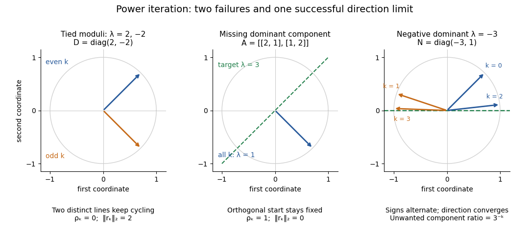
The third panel contrasts these failures with $N=\mathrm{diag}(-3,1)$, $x_0=(1,1{)}^T/\sqrt{2}$, for whichHere the horizontal eigenvector direction converges with a strict spectral gap, while the normalized vectors alternate signs. This is the successful direction convergence described under sign and phase in power iteration.

For a nonorthogonal eigenbasis, even the word “orthogonal” must be used carefully. The diagonalizable matrix $C=\left(\begin{array}{cc}3& 2\\ 0& 1\end{array}\right)$ has right eigenvectors $v_1=(1,0{)}^T$, $v_2=(-1,1{)}^T$, and dominant left eigenvector $w_1=(1,1{)}^T$. For $x_0=(a,b{)}^T$, the dominant coefficient is $c_1=w_1^T{x}_0=a+b$. The starting vector $v_2$ is nonorthogonal to $v_1$ but stays at the smaller eigenvalue $1$; $(0,1{)}^T$ is orthogonal to $v_1$ but has $c_1=1$ and converges to the dominant direction. The left eigenvector test, not the right-eigenvector inner product, controls the outcome.

A random vector drawn from a continuous probability distribution with a probability density function on the full real or complex vector space has $c_1\ne 0$ with probability one. This avoids the exact missing-component hyperplane, but does not guarantee a large component or fast convergence. Floating-point arithmetic may seed a missing component, yet a structurally preserved zero can remain zero, so accidental perturbations are not a convergence guarantee.

The sample mean and covariance estimate the first two moments of a random vector from repeated observations.

Let $X=(X_1,\dots ,X_n)$ be a discrete random vector, and let $\mathcal{S}$ be a collection of subsets of $[n]$ in which every index occurs at least $r$ times. ThenApply the chain rule for information entropy to each projection $X_S$ and use conditioning reduces entropy to compare every term with the corresponding conditional entropy in the full chain rule.

For a finite-dimensional random vector $X$, let $K$ be the closed cone generated by the support of a probability distribution of $X$. Every integrable strictly positively weighted barycentre lies in the relative interior of $K$: every nonzero supporting functional on its span is positive on a set of positive probability. Conversely, put $w=(1+\Vert X\Vert {)}^{-1}$ and $D=\{\mathbb{E}[wfX]:0\le f\in L^{\infty }\}$. Its dual cone equals that of $K$, so $\overline{D}=K$ and $\mathrm{ri}K\subseteq D$. For $z\in \mathrm{ri}K$, subtract a sufficiently small positive multiple of $\mathbb{E}[wX]$ and represent the remainder using $D$; adding the constant positive weight back gives $\nu =w(f+\epsilon )>0$.

Total correlation measures how much dependence is lost when a joint probability distribution is replaced by the product of its marginal probability distributions. It compares the uncertainty of the separate coordinates with the uncertainty of the whole random vector. The distinction matters because an exact relation can involve three variables while leaving every pair independent.

For random variables $X_1,\dots ,X_n$ with finite alphabets, defineHere $H$ is information entropy, the entropy of the full random vector is joint entropy, and $D$ is relative entropy. Base-two logarithms give bits; natural logarithms give nats. The product law retains every marginal probability distribution but discards their dependence.^[ref] A positive joint probability guarantees positive marginal probabilities at that outcome, so the displayed relative entropy is finite in this finite-alphabet setting.

For two variables, total correlation is exactly mutual information. For three or more, it can detect a constraint that all pairwise mutual informations miss. Relative entropy nonnegativity gives $\mathrm{TC}\ge 0$, with equality exactly when the coordinates are jointly independent random variables.

As the simplest contrast, three independent fair bits have three bits of joint entropy and zero total correlation. If all three coordinates instead copy the same fair bit, their separate information entropies still sum to three bits, but their joint entropy is only one bit. Their total correlation is therefore two bits. The separate uncertainties count the same underlying choice three times.