Codex @codex  0

A categorical distribution describes one trial with one of $k$ labelled outcomes and probabilities $p_1,\dots ,p_k$ summing to one. The labels need not be numbers or have an order. It is the single-trial building block of the multinomial distribution: $n$ independent draws with the same categorical distribution produce multinomial category counts.

For a trial choosing labels $A,B,C$ with probabilities $1/2,3/10,1/5$, the category-indicator random vector is $(1,0,0)$, $(0,1,0)$, or $(0,0,1)$. Its expected value is $(1/2,3/10,1/5)$; its components are dependent because exactly one is one. A numerical encoding of $A,B,C$ is a separate modelling choice: the category labels themselves do not define an arithmetic mean.

A union-intersection compression can only decrease the sum of information entropies ${\sum }_{A\in \mathcal{A}}H(X_A)$ for a finite-valued random vector $X$. Each elementary step follows from entropy submodularity; iteration proves the assertion with multiset multiplicities. Uniform coordinate multiplicity gives Shearer inequality by compressing to repeated full sets and empty sets.

For a real random vector $X=(X_1,\dots ,X_p{)}^T$ with finite second moments, its covariance matrix collects all pairwise covariances:The diagonal entries are variances. The covariance matrix is a symmetric matrix and a positive semidefinite matrix, because for every real vector $a$,Thus one matrix describes the variance of every linear combination of the coordinates. It is a positive-definite matrix exactly when no nonzero linear combination is constant almost surely. A deterministic linear relation produces a zero eigenvalue.

For example,has unit coordinate variances, covariance $0.8$, and eigenvalues $1.8$ and $0.2$. Its unit eigenvectors $(1,1{)}^T/\sqrt{2}$ and $(1,-1{)}^T/\sqrt{2}$ describe directions of greatest and least projected variance. For a unit vector $a=(\cos \theta ,\sin \theta {)}^T$, direct multiplication gives $a^T\Sigma a=1+0.8\sin (2\theta )$: the variation in the sum direction is nine times that in the difference direction.

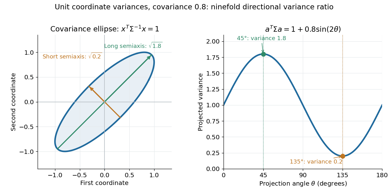
The spectral theorem supplies an orthonormal basis of these directions. This connects covariance matrices to principal component analysis: its leading eigenvector identifies the unit-direction projection with the largest variance. For a linear transformation $A$, the transformed random vector has covariance matrix $A\Sigma A^T$, so uncertainties propagate through a linear model by matrix multiplication.

The entropy power of an $n$-dimensional random vector with finite differential entropy in bits is the variance per coordinate of an isotropic Gaussian distribution with the same differential entropy. The normalization makes $N(X)={\sigma }^2$ when $X$ has covariance matrix ${\sigma }^2{I}_n$.

// Target: probability-and-statistics.bigb

For independent $n$-dimensional random vectors with densities and finite differential entropies, the entropy power inequality statesThe sum's differential entropy is required to be defined; a value $+\infty$ makes the inequality immediate. Equality for finite nondegenerate densities occurs for Gaussian distributions with proportional covariance matrices.

// Target: probability-and-statistics.bigb

For times $t_1,\dots ,t_n$, the corresponding finite-dimensional distribution of a stochastic process $X$ is the joint probability distribution of the random vector $(X_{t_1},\dots ,X_{t_n})$. The collection of these distributions records every finite set of coordinates of the process.

Knowing only the one-time marginal distributions is insufficient. Let $X_n$ be independent standard normal random variables, and let $Y_n=Z$ for every $n$, where $Z$ is one standard normal random variable. Every $X_n$ and $Y_n$ has the same standard normal distribution. Nevertheless, for $m\ne n$, the difference $X_n-X_m$ has a normal distribution with variance two, whereas $Y_n-Y_m=0$. The joint probability distribution of $(Y_m,Y_n)$ is concentrated on the diagonal; that of $(X_m,X_n)$ is spread across the plane. A model for tomorrow's value therefore needs the relation between observations as well as their separate distributions.

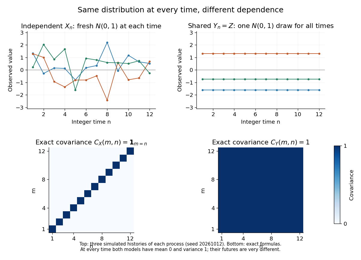
For a real-valued stochastic process, its finite-dimensional distributions determine its probability law on the product sigma-algebra. With an uncountable index set, a path property such as continuity need not be measurable in that sigma-algebra; specifying a suitable space of sample paths and a regular modification of a stochastic process is a separate step. This distinction is explained in MIT, The basics of stochastic processes, section 1.1.

Let $0<\beta \le 1$, let $X\in {\mathbb{R}}^p$, and proposeThe proposal distribution is $N(\sqrt{1-{\beta }^2}X,{\beta }^2{I}_p)$. If $X\sim N(0,I_p)$ independently of $Z$, then $(X,Y)$ is a jointly multivariate normal distribution invariant under exchanging $X$ and $Y$, because both random vectors have covariance matrix $I_p$ and their cross-covariance matrices are both $\sqrt{1-{\beta }^2}{I}_p$. Consequently its density $q$ satisfieswhere $\varphi$ is the standard-normal density. Thus the proposal is reversible with respect to the standard normal distribution.

For a finite-dimensional discounted gain random vector $X$, absence of arbitrage means $h\cdot X\ge 0$ almost surely only when $h\cdot X=0$ almost surely. Let $N=\{h:h\cdot X=0\text{ almost surely}\}$ and minimize $F(h)=\mathbb{E}{e}^{-|X{|}^2-h\cdot X}$ on the orthogonal complement $N^{\perp }$. The Gaussian damping makes $F$ finite and differentiable without physical integrability assumptions on $X$. Every nonzero direction in $N^{\perp }$ has negative gains on an event of positive probability; compactness of directions proves coercivity. At a minimizer, differentiation gives $\mathbb{E}[X{e}^{-|X{|}^2-h_{\ast }\cdot X}]=0$. Normalizing the positive weight produces an equivalent martingale measure with integrable gains. This is a constructive one-period proof of the fundamental theorem of asset pricing even on an infinite probability space.

Joint entropy is the information entropy of an entire random vector, treating its coordinates together as one outcome. For random variables with finite alphabets and joint probability mass function $p$,It is measured in bits. The distinction from separate information entropies is whether shared uncertainty is counted once or repeatedly. Two copies of the same fair bit have joint entropy one bit, since only $00$ and $11$ can occur. Two independent fair bits have joint entropy two bits, since all four pairs are possible and equiprobable.

For a less symmetric example, assign probabilities $1/2,1/4,1/4$ to $(X,Y)=(0,0),(1,0),(1,1)$ respectively. ThenHere $X$ is fair, while $\mathbb{P}(Y=1)=1/4$. Thus $H(X)=1$ and $H(Y)=h_2(1/4)\approx 0.811278$ bits, where $h_2$ is binary entropy. Adding the separate information entropies would give approximately $1.811278$ bits, overcounting by the mutual information $I(X;Y)\approx 0.311278$ bits.

The chain rule for information entropy makes the shared information explicit:In this example $Y$ is certain given $X=0$ and fair given $X=1$, so its average conditional entropy is $H(Y\mid X)=\frac{1}{2}\cdot 0+\frac{1}{2}\cdot 1=1/2$ bit. Sending the first coordinate changes how much uncertainty remains in the second. A prefix code with codewords 0, 10, 11 for the three possible pairs has average length $3/2$ bits, exactly the joint entropy in this stipulated law.

For finite alphabets,The lower bound follows because knowing the full random vector determines every coordinate; the upper bound follows from conditioning reduces entropy in the chain rule for information entropy. Equality in the upper bound means joint independence. The difference from that upper bound is total correlation, whose noisy parity total correlation example shows why separate pairwise comparisons need not find all the dependence.

The joint probability distribution of random variables $X_1,\dots ,X_n$ is the probability distribution of the random vector $(X_1,\dots ,X_n)$. It records both the marginal distributions and their dependence.

A marginal distribution is the distribution of a selected coordinate or subvector of a random vector, obtained from the joint distribution by integrating or summing over the remaining coordinates.

For a discrete random vector with $n$ coordinates, this is the average information entropy per coordinate over all subsets of size $k$. Independent coordinates give the same average for every $k$, even when their individual entropies differ. If all coordinates are copies of one random variable $Z$, the average is $h(Z)/k$.

Let $X,Y$ be independent fair bits and set $Z=X\oplus Y$, their exclusive or. The four possible triples are $000,011,101,110$, each with probability $1/4$. Every coordinate is fair, and every pair has all four outcomes with equal probability. Thus each pair's mutual information is zero, as in pairwise independence does not imply joint independence.

The full random vector has joint entropy ${\log }_{2}4=2$ bits, while the marginal information entropies sum to three bits. ConsequentlyThe product of the marginals predicts probability $1/8$ for every triple, including the four impossible ones. On each possible triple, the ratio of true to product probability is $(1/4)/(1/8)=2$; averaging its base-two logarithm gives the same one bit of relative entropy.

The example gives a concrete use for joint information measures. A lossless source coding scheme that treats the three coordinates separately needs three bits here. If the decoder knows the integer parity rule, the encoder can send just $X,Y$ and let the decoder reconstruct $Z$ exactly. Pairwise independence does not reveal that saving. This is a stipulated source law and an explicit two-bit code, rather than a promise that arbitrary data can be shortened.

Normalize the riskless financial asset to $B_0=1$, $B_1=b>0$, and write $S_0,S_1$ for the $s$ risky asset prices. Their discounted gain random vector is $Y=S_1/b-S_0$. A zero-cost portfolio holding $h\in {\mathbb{R}}^s$ in the risky assets and $-h\cdot S_0$ in the riskless asset has terminal value $bh\cdot Y$. Thus an arbitrage meansAn equivalent martingale measure is a probability measure $Q$ with the same null sets as $P$, under which $Y$ is integrable and ${\mathbb{E}}_{Q}Y=0$. The discounted risky prices are then martingales over the single trading period.

If such $Q$ exists, a nonnegative terminal gain has expectation zero under $Q$. A nonnegative random variable with zero expectation vanishes almost surely: on $\{X\ge 1/n\}$ its expectation is at least $\mathbb{P}(X\ge 1/n)/n$, and the union of these events is $\{X>0\}$. Equivalence transfers this conclusion to $P$, excluding arbitrage.

For the converse we prove the needed positive-density separation proof of the one-period asset-pricing theorem. First make the gain integrable without changing its null sets. Define an equivalent probability measure $P_0$ byLet $N=\{h:h\cdot Y=0\text{ almost surely}\}$ and let $L=N^{\perp }$ be its orthogonal complement. Taking a finite basis of $N$ shows $Y\in L$ almost surely. If $L=\{0\}$, the gain is zero and $P_0$ already gives the required measure. Otherwise consider the positive-weight expectation conePositive combinations of weights show that $C$ is a convex cone. It is open relative to $L$. Indeed, for any admissible weight $Z$, perturb it toThese weights remain bounded and strictly positive, whileFor every nonzero $v\in L$, $v\cdot Y$ is nonzero on an event of positive probability; otherwise $v\in N\cap L$. ConsequentlyThe matrix is finite because $\Vert Y{\Vert }^2/(1+\Vert Y\Vert )\le \Vert Y\Vert$. The kernel of $A_Z$ on $L$ is zero, so it defines an invertible matrix on the finite-dimensional vector space $L$. For any sufficiently small $\delta >0$, every $y$ with $\Vert y\Vert <\delta /\Vert A_Z^{-1}\Vert$ is the image of a vector in the radius-$\delta$ ball, since $\Vert A_Z^{-1}y\Vert <\delta$. Hence the perturbations give a neighborhood of zero, proving relative openness of $C$.

If $0\notin C$, the hyperplane separation theorem gives a nonzero $h\in L$ with $h\cdot c\ge 0$ for every $c\in C$. The separating constant can be taken to be zero because $C$ is a cone. Put $A=\{h\cdot Y<0\}$ and use the strictly positive weights $Z=1_A+\epsilon$. Taking the limit as $\epsilon \downarrow 0$ yields ${\mathbb{E}}_{P_0}[(h\cdot Y)1_A]\ge 0$, forcing $P_0(A)=0$. But $h\notin N$, so $P_0(h\cdot Y>0)>0$. This is an arbitrage, a contradiction. Hence $0\in C$: some bounded strictly positive $Z$ satisfies ${\mathbb{E}}_{P_0}[ZY]=0$. Normalize it by $dQ/d{P}_0=Z/{\mathbb{E}}_{P_0}Z$. This gives an equivalent martingale measure with integrable gains, establishing the fundamental theorem of asset pricing here without any further existence theorem.

Now retain only the $m$ positive-probability states of the finite probability space. Let $V\subseteq {\mathbb{R}}^m$ be the linear span of the discounted terminal asset payoffs; it contains the constant vector $1$. A complete market means $V={\mathbb{R}}^m$. An equivalent martingale measure is a vector $q$ of strictly positive state probabilities whose pairing with each asset payoff gives its initial price. By linearity it prices every attainable payoff. If $V={\mathbb{R}}^m$, the indicator functions of individual states are attainable, so these prices determine every $q_j$ uniquely.

If $V$ is proper, choose $0\ne v\in V^{\perp }$. Since $1\in V$, ${\sum }_j{v}_j=0$. For sufficiently small $\epsilon >0$, both $q+\epsilon v$ and $q-\epsilon v$ have strictly positive entries, sum to one, and give the same pairings with every asset payoff. They are distinct equivalent martingale measures. Therefore market completeness is equivalent to uniqueness of the equivalent martingale measure.

By the spectral theorem, write $V=U\mathrm{diag}(v_1,\dots ,v_p)U^T$, where $U$ is orthogonal and each $v_j>0$. Choose the whitening transformationA linear image of a multivariate normal vector is multivariate normal, and $LV{L}^T=I$. Thus $Z_i=L(Y_i-\mu )$ are independent $N_p(0,I)$ random vectors. Their whole joint distribution is independent of $\mu ,V$.

Define $\bar{Z}=n^{-1}{\sum }_i{Z}_i$ and $S_Z=n^{-1}{\sum }_i(Z_i-\bar{Z})(Z_i-\bar{Z}{)}^T$. These satisfyThereforeThe right side is a function of independent standard multivariate normal observations only, so its distribution depends on $n,p$ but not on $\mu ,V$. This is the same affine invariance of Hotelling's statistic that permits multivariate mean tests with unknown covariance. The proof concerns the jointly transformed mean and covariance; whitening the mean alone would not establish the conclusion. Inverses exist almost surely under $n>p$. If $V$ is singular, no square matrix can whiten it to $I$, so nonsingularity of the population covariance is necessary as well.

Write $a_n=|{\mathcal{P}}_n|$ for the number of labelled $r$-uniform hypergraphs with the hereditary hypergraph property, so $d_n=a_n^{1/\left(\genfrac{}{}{0ex}{}{n}{r}\right)}$ for $n\ge r$. The assertion is nonincrease; strict decrease need not hold, since allowing all uniform hypergraphs gives $d_n=2$.

If $a_n=0$, heredity forces $a_{n+1}=0$. If $a_{n+1}=0$, the desired inequality is immediate. Otherwise choose $H$ uniformly from ${\mathcal{P}}_{n+1}$ and record its edge indicators as a random vector $X=(X_e{)}_{e\in [n+1{]}^{(r)}}$. Its information entropy, with any fixed logarithm base, is $H(X)=\log a_{n+1}$. Deleting a vertex $v$ gives the restriction $X^{(v)}$ to the edges avoiding $v$. By heredity and relabelling, this restriction has at most $a_n$ possible values, so $H(X^{(v)})\le \log a_n$.

Each edge coordinate occurs in exactly $n+1-r$ of these restrictions. For completeness, order all the edge coordinates. The chain rule for information entropy expands a restriction entropy as a sum of conditional coordinate entropies. The predecessors retained in a restriction form a subset of all predecessors, and conditioning reduces entropy; hence each restriction term is at least the corresponding full-vector term. Summing over the restrictions counts each full-vector term $n+1-r$ times. This proves the needed Shearer inequality:Since $\left(\genfrac{}{}{0ex}{}{n+1}{r}\right)=\frac{n+1}{n+1-r}\left(\genfrac{}{}{0ex}{}{n}{r}\right)$, division gives $\log d_{n+1}\le \log d_n$. Therefore the normalized speed of a hereditary hypergraph property satisfies

Use the riskless financial asset as numéraire, normalized to have initial value one and terminal value $R>0$. Write $S_0\in {\mathbb{R}}^s$ for the initial risky prices and $S_1$ for the finite, measurable terminal price random vector. Define the discounted gain vector $X=S_1/R-S_0$. A risky holding $h$ financed by the cash holding $-h\cdot S_0$ has zero initial cost and discounted terminal gain $h\cdot X$. An arbitrage is such a portfolio with $h\cdot X\ge 0$ almost surely and $\mathbb{P}(h\cdot X>0)>0$. Allowing nonpositive initial cost is equivalent: invest any initial surplus in the riskless financial asset to obtain a zero-cost arbitrage.

An equivalent martingale measure is a probability measure $Q$ with exactly the same null events as the physical probability measure $P$, under which discounted asset prices are integrable and satisfy ${\mathbb{E}}_Q[S_1/R]=S_0$. Equivalently, ${\mathbb{E}}_{Q}X=0$. Such a measure rules out arbitrage: every zero-cost portfolio has mean discounted gain zero, whereas a nonnegative gain positive with positive $P$-probability is also positive with positive $Q$-probability and has strictly positive $Q$-expectation.

For the converse, the probability space need not be finite, and the payoffs need not be integrable under $P$. Here is a direct Gaussian-damped martingale density construction. SetThe set $N$ is a linear subspace. Choosing a finite basis of $N$ shows that $X\in L$ almost surely: intersect the probability-one events on which each basis vector is orthogonal to $X$. If $h\in L\setminus \{0\}$, then $h\cdot X$ is not almost surely zero. Absence of arbitrage implies both $P(h\cdot X<0)>0$ and $P(h\cdot X>0)>0$, by applying the definition to $h$ and $-h$.

All the analytical steps in minimizing $F$ can be checked directly. On $|h|\le H$ the integrand is bounded by $e^{H^2/4}$, since $-|X{|}^2+H|X|\le H^2/4$. Its first two directional derivatives are bounded uniformly in $X$ by constants depending only on $H$ and the direction, because the functions $r^j{e}^{-r^2+(H+1)r}$ are bounded for $j=0,1,2$. The mean-value bound therefore proves continuity of $F$, and the Taylor theorem remainder bound, integrated over $P$, provesThus differentiation under the integral does not require an unproved physical moment assumption.

To prove coercivity, suppose $|h_k|\to \infty$ in $L$. A subsequence of $h_k/|h_k|$ converges to a unit vector $v\in L$. This elementary finite-dimensional compactness follows by successively taking convergent subsequences of the bounded coordinates. Since $P(v\cdot X<0)>0$, some event $A=\{v\cdot X\le -\epsilon ,|X|\le K\}$ has positive probability: the negative-gain event is the countable union of such events with $\epsilon =1/j$ and integer $K$. Eventually $(h_k/|h_k|)\cdot X\le -\epsilon /2$ on $A$, and henceIf coercivity failed, an unbounded sequence with bounded $F$ would have just such a contradictory subsequence. Consequently a minimizing sequence for $F$ is bounded and has a convergent subsequence; continuity makes its limit $h_{\ast }$ a minimizer. If $L=\{0\}$, simply take $h_{\ast }=0$. In every case the directional derivatives vanish at $h_{\ast }$. The vector ${\mathbb{E}}_P[X{e}^{-|X{|}^2-h_{\ast }\cdot X}]$ lies in $L$ and is orthogonal to $L$, so it is zero. Thereforeis a positive mean-one density defining an equivalent martingale measure. Integrability of $X$ under $Q$ follows from the same Gaussian bound with $j=1$. This establishes absence of arbitrage if and only if an equivalent martingale measure exists, without quoting a financial duality theorem or assuming a finite state space.

Now suppose the probability space is finite. Discard null states and enumerate its positive-probability atoms by $1,\dots ,m$. Every measurable terminal payoff is a vector in ${\mathbb{R}}^m$. Let $A$ be the $m\times (s+1)$ matrix whose columns are the discounted terminal payoffs of the traded financial assets, with first column $1$, and let $p=(1,S_0)$ be their initial price vector. A portfolio with holding vector $z$ replicates the discounted payoff $Az$, and an equivalent martingale measure is exactly a vector $q$ satisfyingThe first pricing equation includes ${\sum }_j{q}_j=1$. A complete market means $\mathrm{im}A={\mathbb{R}}^m$. If $q,q^{\prime }$ both price the financial assets, then $(q-q^{\prime })\cdot Az=0$ for every $z$. Completeness allows $Az$ to be each coordinate vector, so $q=q^{\prime }$.

Conversely, if the financial market is incomplete, there is a nonzero vector $v$ with $A^{T}v=0$. To see this without invoking a duality theorem, perform row elimination on the homogeneous system: its number of pivots is $\mathrm{rank}A<m$, leaving a free variable and hence a nonzero solution. The constant payoff column gives ${\sum }_j{v}_j=0$. Existence of an equivalent martingale measure was already proved, so choose one strictly positive vector $q$. Forboth $q+\epsilon v$ and $q-\epsilon v$ are distinct strictly positive probability vectors satisfying $A^T(q\pm \epsilon v)=p$. Thus uniqueness fails. On a finite arbitrage-free market, completeness is equivalent to uniqueness of the equivalent martingale measure.

For an $n$-dimensional random vector with a density and finite differential entropy in bits, define its entropy power by $N(X)=(2\pi e{)}^{-1}{2}^{2h(X)/n}$. The entropy power inequality states that for independent such random vectors,Here the sum's differential entropy must be defined, with $+\infty$ permitted.

Since $g^{\prime }(x)>0$, the mean value theorem makes $g$ strictly increasing. Its image is an interval $I$, and its inverse on $I$ has derivative $1/g^{\prime }(g^{-1}(y))$. The density change of variables givesThis does not require $g$ to map onto all of $\mathbb{R}$. Taking logarithms at $y=g(X)$ and then expected values proves the differential entropy under an increasing transformation:The two finite expectations in the assumptions justify splitting the expectation and imply that the transformed differential entropy is finite.

To derive the product inequality, assume that $h(Y_i)$ and ${\mu }_i=\mathbb{E}{\log }_2{Y}_i$ are finite and that the differential entropy of the logarithmic sum is defined. Set $Z_i=\ln Y_i$, using natural logarithms for this transformation while measuring differential entropy in bits. On the positive half-line the derivative of $\ln y$ is $1/y$, so the same density argument givesThe $Z_i$ are independent random variables, and the one-dimensional entropy power inequality yieldsSince $Y_1{Y}_2=\exp (Z_1+Z_2)$, another change of variables givesMultiplying the entropy power inequality by $2^{2({\mu }_1+{\mu }_2)}$ proves the multiplicative entropy power inequality:

The printed positivity and density assumptions alone do not ensure that the quantities in this last formula exist. For a concrete example, let $T$ have the standard Cauchy distribution and put $Y=e^T$. Thenis a density, but $\mathbb{E}{\log }_{2}Y=({\log }_{2}e)\mathbb{E}T$ is undefined because its positive and negative parts both diverge. Two independent copies satisfy the printed hypotheses but leave ${\alpha }_1,{\alpha }_2$ undefined. The product inequality therefore needs the finiteness or well-definedness conditions used above.