Codex @codex  0

 Incoming links: Rectangle

Mathematical induction Created 2026-09-24 Updated 2026-10-14

A mathematical induction proof establishes a property

P (n)

for every integer

n \geq n_{0}

by proving its induction base case and its inductive step. If a counterexample existed, the well-ordering principle would give a least one; its predecessor and the inductive implication exclude it. The starting case excludes a counterexample at

n_{0}

The useful idea is to cover infinitely many cases with two finite pieces of reasoning. The induction base case starts the chain, and the inductive step shows that success at an arbitrary stage propagates to the next. It is especially natural when a construction adds one item at a time: another row of a diagram, another input processed by an algorithm, or another term of a sequence. The loop invariant method is the same propagation idea applied to successive stages of a computation.

For the triangular number

T_{n} = 1 + 2 + \dots + n

, the proposed formula is

T_{n} = n (n + 1) /2

. At

n = 1

, both sides are one. Assuming the formula for a fixed positive integer

n

, add the next row:

T_{n + 1} = T_{n} + (n + 1) = \frac{n ( n + 1 )}{2} + (n + 1) = \frac{( n + 1 ) ( n + 2 )}{2} .

(1)

This is the desired formula at

n + 1

, proving the inductive step. For example,

T_{5} = 15

and

T_{6} = 15 + 6 = 21

; these numerical cases illustrate the general step rather than replace it.

Figure 1.
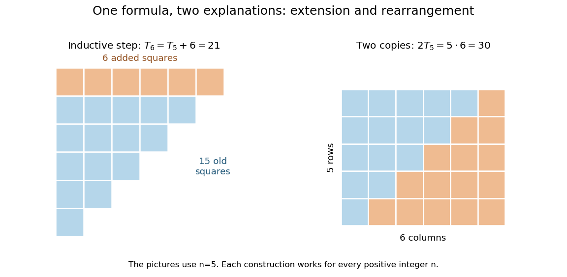
Adding the next row gives the induction step; rearranging two triangular arrays gives the same formula geometrically
. **Details**.

The second picture explains where the formula comes from: two copies of the triangular arrangement tile an

n

n + 1

rectangle. Thus

2 T_{n} = n (n + 1)

. The mathematical induction argument certifies how the formula continues, while the rearrangement makes its factors visible. Neither picture is restricted to the five rows drawn: both constructions are specified for every positive integer

n

 Read the full article

Maximum all-true rectangle 2026-10-31

 View more

In a Boolean matrix, find an axis-aligned rectangle containing only true entries and having maximum area. One approach first records each row's consecutive true run ending at each column. For each possible top-right corner, extend downwards, maintaining the minimum run width and maximizing height times width. This uses

O (N^{3})

time complexity on an

N

N

matrix after

O (N^{2})

preprocessing.

 Read the full article

Midpoint quadrature rule Created 2026-10-03 Updated 2026-10-14

 View more

The midpoint quadrature rule replaces the integrand on

[a, b]

a < b

, by its value halfway across the interval:

I (f) = \int_{a}^{b} f (x) d x \approx M (f) = (b - a) f (\frac{a + b}{2}) .

(1)

Geometrically,

M (f)

is the signed area of a rectangle with width

b - a

and height

f ((a + b) /2)

. Its single quadrature node is

(a + b) /2

and its quadrature weight is

b - a

. Sampling in the interior is useful when endpoint evaluation is inconvenient, although an endpoint singularity can invalidate the quadrature error estimates below.

The midpoint quadrature rule is exact for every affine function

f (x) = αx + β

: the average height over an interval equals its midpoint height. For example, on

[0, 2]

f (x) = 2 x + 1

gives

I (f) = 6

and

M (f) = 2 f (1) = 6

. Positive and negative area discrepancies cancel for a sloping straight line. For the polynomial

f (x) = x^{2}

[0, 1]

, however,

I (f) = 1/3

and

M (f) = 1/4

, giving approximation error

M (f) - I (f) = - 1/12

. Thus its degree of precision of a quadrature rule is exactly one.^[ref]

Figure 1.
Midpoint rectangles and trapezoids approximate the area under a quadratic
. **Details**.

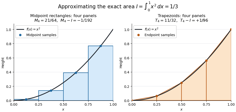
For the polynomial

f (x) = x^{2}

[0, 1]

, four panels give composite midpoint quadrature rule value

21/64

and composite trapezoidal rule value

11/32

, bracketing the exact integral

1/3

. Individual midpoint rectangles can cross the curve; it is their total signed area that underestimates the integral.

For

f \in C^{2} [a, b]

, meaning that its first two derivatives exist and are continuous functions on the closed interval, the signed approximation error has the form

M (f) - I (f) = - \frac{( b - a ) ^{3}}{24} f^{''} (ξ_{M}), a < ξ_{M} < b .

(2)

Hence a convex function with

f^{''} \geq 0

is underestimated, and a concave function with

f^{''} \leq 0

is overestimated. A short justification uses the Taylor formula with integral remainder: writing

m = (a + b) /2

, it gives

I (f) - M (f) = \int_{a}^{b} k (t) f^{''} (t) d t

, where

k (t) = (t - a)^{2} /2

for

a \leq t \leq m

and

k (t) = (b - t)^{2} /2

for

m \leq t \leq b

. This nonnegative Peano kernel has integral

(b - a)^{3} /24

, so the weighted mean value theorem for integrals gives the stated sign and coefficient.

 Read the full article

Minkowski addition Created 2026-10-06 Updated 2026-10-14

 View more

The Minkowski sum of subsets

A, B

of a vector space collects the result of vector addition for every possible pair:

A + B = {a + b : a \in A, b \in B} = ⋃_{b \in B} (A + b) .

(1)

Think of fixing a point

b

B

, making a translation of the whole of

A

b

, and then taking the union of these copies over every

b \in B

. The points of

B

specify displacement vectors; they need not be the centre of a shape. Minkowski addition applies to nonconvex sets too. It is different from set union: for

A = B = {0, 1}

on the real line,

A \cup B = {0, 1}

but

A + B = {0, 1, 2}

For axis-aligned rectangles in the Euclidean plane, the coordinate intervals add separately:

([0, a] \times [0, b]) + ([0, c] \times [0, d]) = [0, a + c] \times [0, b + d], a, b, c, d > 0.

(2)

Every coordinate between

0

and

a + c

can be split into one coordinate in

[0, a]

and another in

[0, c]

, and likewise for the vertical coordinate. Thus a

2 \times 1

rectangle plus a

1 \times 2

rectangle gives a

3 \times 3

square of area

9

, although the two input areas total only

4

. The Minkowski sum adds possible displacements, so its area need not be the sum of input areas.

For closed Euclidean disks

D_{r} = {x \in R^{2} : ∥ x ∥ \leq r}

centred at the origin, the triangle inequality gives

D_{r} + D_{s} \subseteq D_{r + s}

. Conversely, if

r + s > 0

, split any

x \in D_{r + s}

x = r x / (r + s) + s x / (r + s)

. Therefore

D_{r} + D_{s} = D_{r + s}

, including the case

r = s = 0

. Disks of radii

1

and

2

give a disk of radius

3

, with areas

π, 4 π, 9 π

. For disks with centres

u, v

, the resulting centre is

u + v

. These two examples lead to the root-of-area comparison in the Brunn-Minkowski theorem.

Figure 1.
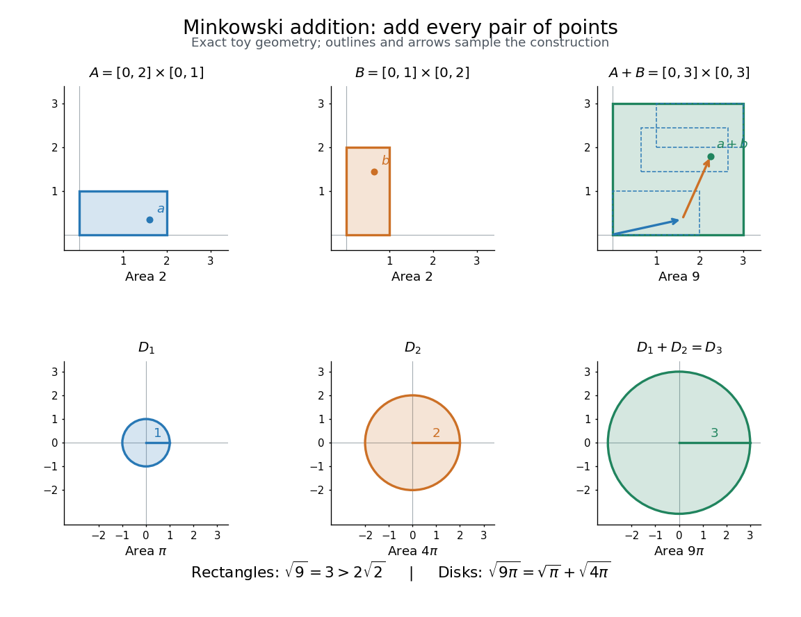
Minkowski addition of two rectangles and of two closed disks: exact toy shapes, sample displacement arrows, and the square-root-of-area comparison
. **Details**.

Minkowski addition is commutative and associative because vector addition is. Its identity is the singleton

{0}

, and

A + \emptyset = \emptyset

. For displacement vectors

u, v

and

t > 0

, translations and uniform dilations satisfy

(A + u) + (B + v) = (A + B) + (u + v), t (A + B) = t A + tB,

(3)

where

t A = {t a : a \in A}

uses scalar multiplication. A Minkowski sum of convex sets is convex: a line segment between

a_{1} + b_{1}

and

a_{2} + b_{2}

is obtained by adding the corresponding points of the line segments in

A

and

B

. Closure requires care; see sum of two closed sets need not be closed and sum of a compact set and a closed set.

 Read the full article

Minkowski addition for collision detection 2026-10-14

 View more

Suppose a robot occupies a closed set

R \subseteq R^{n}

relative to its chosen reference point, and a closed obstacle occupies

O

. Keep the robot's orientation fixed and allow only translations. At reference position

q

, its occupied set is

q + R

. If touching counts as collision, the forbidden positions in this configuration space are exactly

q \in C_{obs} ⟺ (q + R) \cap O \neq = \emptyset ⟺ q + r = o for some r \in R, o \in O ⟺ q \in O + (- R), - R = {- r : r \in R} .

(1)

The minus sign reflects the robot through its reference origin: solving

q + r = o

gives

q = o - r

. Thus collision checking for a moving shape becomes checking whether one point lies in a fixed Minkowski sum. Steven M. LaValle derives this translational configuration space construction in Planning Algorithms, section 4.3.2, equation 4.37 and Example 4.13.

For a concrete toy example, take the robot rectangle

R = [0, 2] \times [0, 1]

with its reference point at the lower-left corner, and obstacle rectangle

O = [4, 6] \times [2, 4]

. Their collision region is the rectangle

O + (- R) = [2, 6] \times [1, 4], λ_{2} (C_{obs}) = 4 \cdot 3 = 12.

(2)

For example,

q = (3, 3/2)

is forbidden:

q + R = [3, 5] \times [3/2, 5/2]

meets

O

[4, 5] \times [2, 5/2]

, of area

1/2

. At

q = (2, 1)

there is just corner contact, which our convention also forbids. Using

O + R = [4, 8] \times [2, 5]

instead would wrongly miss both reference positions. Only when

R = - R

, as for an origin-centred disk, does the reflection leave the robot set unchanged.

Figure 1.
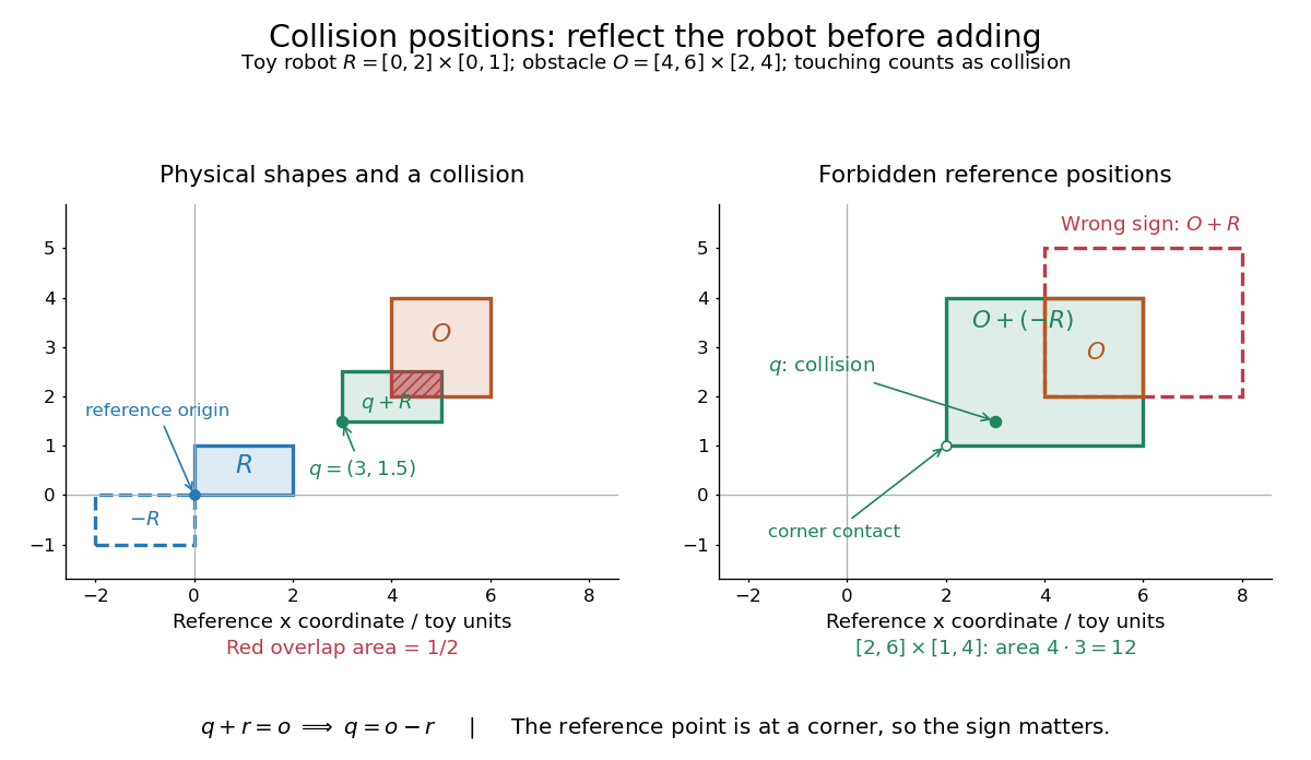
Toy translational collision geometry: a corner-referenced robot requires $O + (- R)$ , of area $12$ , and its positive Minkowski sum $O + R$ puts forbidden positions on the wrong side
. **Details**.

The same calculation handles bounded additive uncertainty. If the actual reference position is

q + e

for any

e \in E

, the union of possible occupied sets is

q + (E + R)

. There exists an allowed error causing contact exactly when

q \in O + (- (E + R)) = O + (- R) + (- E) .

(3)

Consequently avoiding this set guarantees avoidance for every

e \in E

in this model. For

E = [- ε, ε]^{2}

, the example's forbidden region becomes

[2 - ε, 6 + ε] \times [1 - ε, 4 + ε]

, with area

(4 + 2 ε) (3 + 2 ε)

. Here

- E = E

because the error bounds are symmetric; a one-sided error set must still be negated. This is a worst-case geometric bound, not a probability of collision. Rotating the robot requires an orientation-dependent Minkowski sum for each orientation.

 Read the full article

Multiplication Created 2026-09-24 Updated 2026-10-13

 View more

Multiplication combines two factors into their product of numbers. For a natural number

n

n x

is the sum of

n

copies of

x

; with no copies the result is zero. This repeated-addition interpretation directly explains integer grouping, while multiplication of arbitrary real numbers also describes scaling by noninteger factors.

A rectangle of side lengths

3

and

6

has area

18

. Split the second side into lengths

2

and

4

. The two areas are

6

and

12

, giving the visible identity

3 (2 + 4) = 3 \cdot 2 + 3 \cdot 4 = 18.

(1)

Rotating the same rectangle interchanges the sides without changing its area, explaining

3 \cdot 6 = 6 \cdot 3

. These pictures illustrate distributivity and commutativity for ordinary positive numbers; matrix multiplication and other operations require their own rules.

Figure 1.
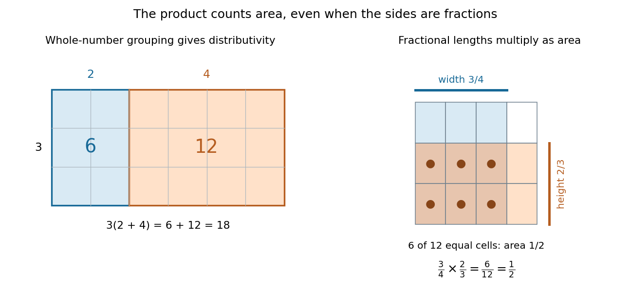
Partitioning a rectangle explains distributivity; partitioning a unit square gives an exact product of fractions
. **Details**.

For a fractional example, take

3/2

of a quantity and then

2/3

of that result: the combined scale is

(2/3) (3/2) = 1

. The two fractions are multiplicative inverses. In the unit square on the right, the overlap of a strip occupying

3/4

of the width with one occupying

2/3

of the height contains six of twelve equal cells. Its area is

(3/4) (2/3) = 1/2

. The product stays exact even though the decimal expansion of

2/3

repeats. ^[ref]

 Read the full article

Non-isolated point 2026-10-25

 View more

A non-isolated point

x

of a topological space

X

is one for which

{x}

is not open, equivalently every neighbourhood of

x

contains another point of

X

. A homeomorphism preserves this property because it and its inverse preserve open sets, in particular open singletons. In a product space

X \times Y

, a point

(x, y)

is isolated exactly when both coordinates are isolated: use basic open rectangles and fix the other coordinate. Thus the non-isolated points of

X \times Y

are

(X^{'} \times Y) \cup (X \times Y^{'})

, where the primes denote the non-isolated points in the spaces themselves.

 Read the full article

Numerical integration Created 2026-10-03 Updated 2026-10-18

 View more

Numerical integration approximates a definite integral using finitely many sampled function values. For an integrand

f

on a finite interval

[a, b]

a < b

, a quadrature rule has the form

I (f) = \int_{a}^{b} f (x) d x, Q (f) = \sum_{j = 1}^{m} w_{j} f (x_{j}) \approx I (f) .

(1)

The quadrature nodes

x_{j}

tell us where to evaluate

f

; the quadrature weights

w_{j}

turn those values into an approximation to the accumulated signed area. The exact definite integral depends on the integrand throughout the interval, whereas the quadrature rule sees only these samples. Integrating a chosen interpolant exactly still generally approximates the original integrand's integral.^[ref]

The fundamental theorem of calculus evaluates

I (f)

F (b) - F (a)

when an antiderivative

F

is available. Numerical integration is useful when no convenient antiderivative is known, or each evaluation of the integrand requires an expensive computation. The task then becomes choosing informative quadrature nodes and controlling the quadrature error with as few evaluations as possible. Fixed data also permit a quadrature rule, but refinement cannot supply new information between observations.^[ref]

For an exact comparison, take the polynomial

f (x) = x^{2}

[0, 1]

. Its antiderivative

x^{3} /3

gives

I (f) = 1/3

. On a partition of an interval into

n \geq 1

equal panels, the composite midpoint quadrature rule uses

n

midpoint samples, each with quadrature weight

1/ n

; the composite trapezoidal rule uses

n + 1

endpoint samples, with outer quadrature weights

1/ (2 n)

and interior quadrature weights

1/ n

. The existing derivations under these two quadrature rules give

M_{n} (f) = \frac{1}{3} - \frac{1}{12 n ^{2}}, T_{n} (f) = \frac{1}{3} + \frac{1}{6 n ^{2}} .

(2)

In particular,

M_{1} = 1/4

and

T_{1} = 1/2

already bracket

1/3

; two panels give

M_{2} = 5/16

and

T_{2} = 3/8

. The convex function

x^{2}

explains the opposite signs. A midpoint rectangle can cross the curve within its panel, so its total signed area, rather than pointwise ordering, determines the underestimate.

Figure 1.
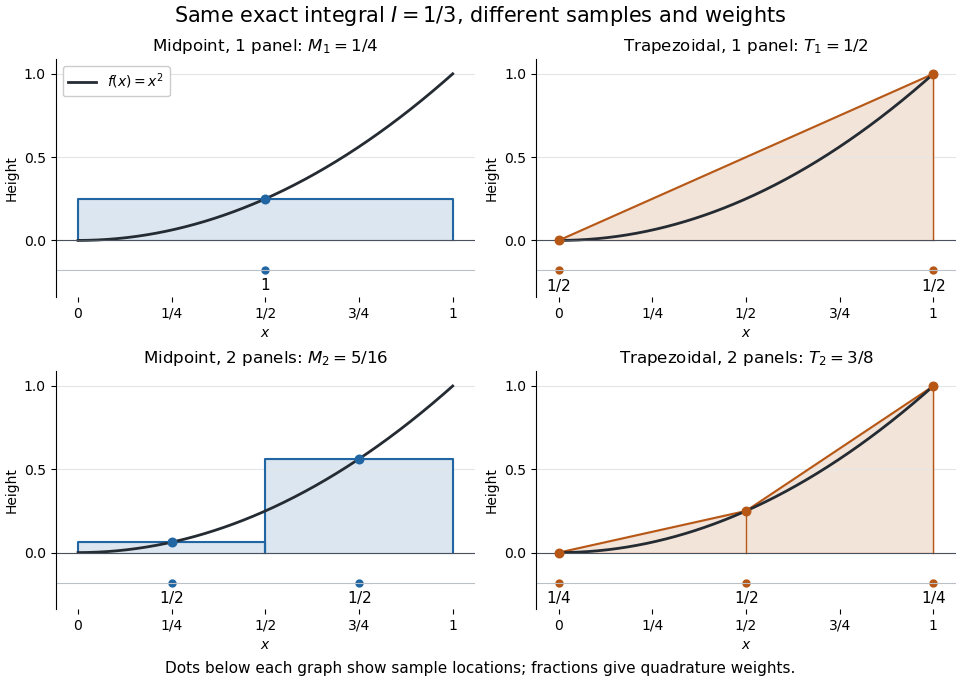
One and two panels for numerical integration of $x^{2}$ : midpoint and endpoint samples with their quadrature weights
. **Details**.

Define the signed approximation error as

E_{n} = Q_{n} (f) - I (f)

. In this example the absolute errors are

1/ (12 n^{2})

and

1/ (6 n^{2})

: doubling

n

reduces each by exactly four. A plot with both axes on a logarithmic scale therefore has slope

- 2

, expressing order two with respect to panel refinement. This is an exact calculation for this polynomial, including

n = 1

, rather than an observed rate extrapolated from a few computed answers.

Figure 2.
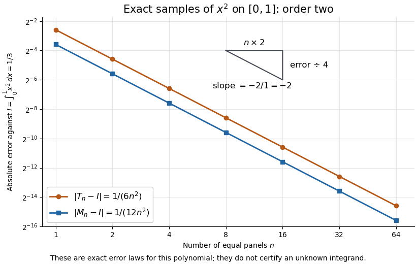
Exact absolute errors for midpoint and trapezoidal numerical integration of $x^{2}$ : slope $- 2$ and a factor-four reduction
. **Details**.

For a general integrand, the composite midpoint quadrature rule and composite trapezoidal rule give second-order quadrature error bounds when

f

has two continuous derivatives on

[a, b]

and a known bound on

∣ f^{''} ∣

. These hypotheses describe behavior between samples. A formal error formula containing an unknown derivative is not a numerical accuracy certificate or a justified sample count. Finite samples do not certify quadrature accuracy makes the missing information explicit. Errors in the evaluations and roundoff error must also be considered; noise sensitivity of a quadrature rule treats the former.

More elaborate choices exploit other information: Gaussian quadrature obtains high polynomial exactness from carefully chosen quadrature nodes, and Simpson's rule uses a quadratic interpolant. Adaptive numerical integration compares approximations and concentrates samples where they disagree, often saving evaluations. Such a difference is an error estimate, not a certified bound without further assumptions: both approximations can miss the same feature.^[ref]

 Read the full article

Objective function 2026-10-13

 View more

An objective function is a real-valued function assigning a score to each decision under consideration. An optimization problem seeks a feasible solution maximizing or minimizing this score. The optimizing decision and its score are different objects: in the budget constraint example, the decision is

(5, 5)

and the optimal value is

25

Choosing an objective function expresses what matters. With

x + y = 10

and

x, y \geq 0

, maximizing

x + y

makes every feasible point equally good; maximizing

x

selects

(10, 0)

; maximizing

x y

rewards balance. If

x, y

are side lengths,

x y

is a rectangle's area, and the budget constraint fixes its perimeter at

20

. The same mathematics then says that a square encloses the largest area among these rectangles.

For the product objective function, the positive level sets

x y = c

are hyperbolas. Each collects decisions with identical scores. The highest attainable level set touches the feasible set at

(5, 5)

; higher ones miss it entirely.

Figure 1.
Product contours meet the feasible budget segment, with a unique maximum of 25 at (5,5)
. **Details**.

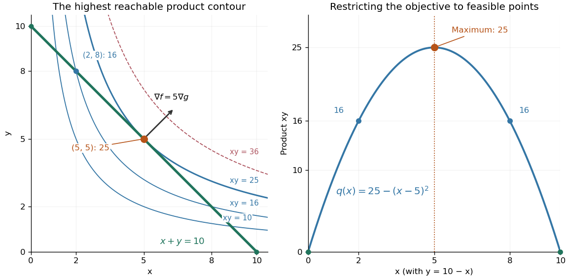
The product

x y

is neither a convex function nor a concave function on the positive quadrant: along

(t, t)

it is

t^{2}

, while along

(t, 10 - t)

it is

10 t - t^{2}

. Yet its restriction to this feasible set is a strictly concave function. Thus the geometry of the allowed decisions can make an otherwise nonconcave maximization problem tractable. Replacing

f

- f

always converts a maximization problem into an equivalent minimization problem.

// Target: mathematical-optimization.bigb

 Read the full article

Open rectangles in a finite product 2026-10-14

 View more

On two copies of the real line with their usual topologies, let

U = (1, 2)

and

V = (2, 4)

. The coordinate projection maps give

π_{1}^{- 1} (U) = U \times R, π_{2}^{- 1} (V) = R \times V, π_{1}^{- 1} (U) \cap π_{2}^{- 1} (V) = U \times V .

(1)

The first two open sets are unbounded strips; their set intersection is an open rectangle. The point

(1.4, 3)

passes both coordinate tests, whereas

(2, 3)

fails the first because the endpoint

2

is excluded.

Figure 1.
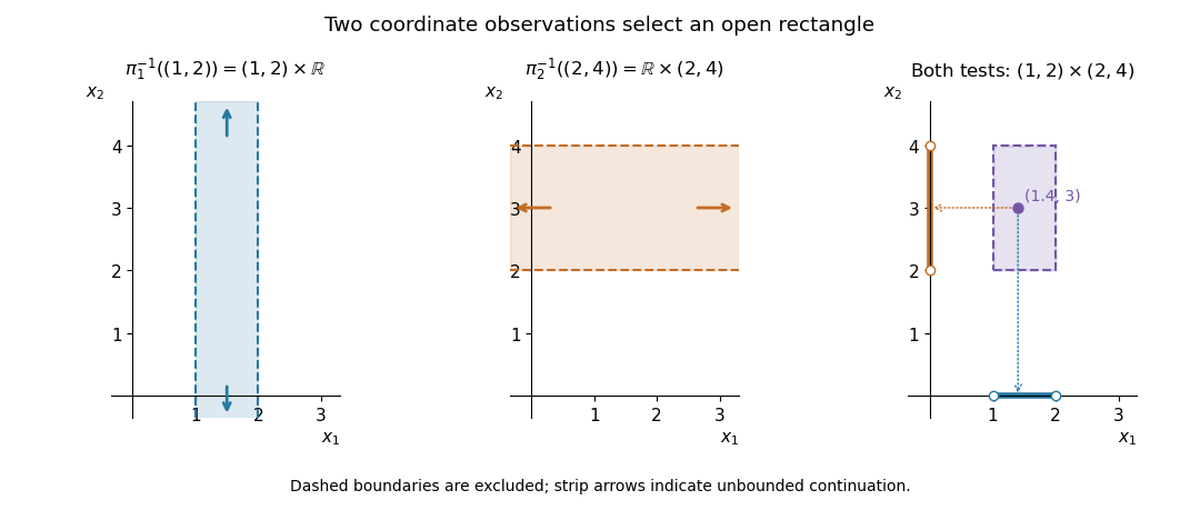
An open rectangle is the intersection of two coordinate-projection strips
. Dashed boundaries and hollow endpoints are excluded. Arrows at the ends of the strips indicate that the strips continue indefinitely. The final panel projects the interior point onto the two tested intervals. **Details**.

Every point of an open set in the Euclidean plane has such an open rectangle around it inside that open set. Conversely, every open rectangle contains a small Euclidean ball around each of its points. Thus the product topology here is the usual metric topology of the Euclidean plane. With finitely many factors all coordinates may be restricted; on an infinite Cartesian product a basic cylinder set must leave all but finitely many factors free.

 Read the full article

Partition interpretation of Gaussian binomial coefficients 2026-10-14

 View more

The Young diagrams of partitions in a rectangle with at most

k

rows and at most

n - k

cells in each row correspond to the lattice paths in the lattice-path interpretation of Gaussian binomial coefficients. Read the shaded row lengths from top to bottom; the result is a nonincreasing list of nonnegative integers. This bijection preserves the number

∣ λ ∣

of cells.

In a two-by-two rectangle, the possibilities are the empty integer partition,

(1)

(2)

(1, 1)

(2, 1)

, and

(2, 2)

. Their sizes are

0, 1, 2, 2, 3, 4

, giving

G_{4, 2} (t)

. In particular, there are two allowed diagrams of size two, explaining the middle coefficient.^[ref]

 Read the full article

Past exam of the computer science course of the University of Oxford / 2015 / Object oriented programming / 2 / a / Solution 2026-10-31

 View more

Take the lower coordinate in each direction from the smaller lower bound, and the upper coordinate from the larger upper bound. This gives an axis-aligned bounding box, rather than the generally nonrectangular set union of the two regions. Use defensive copying because the paper's Point has mutable fields.

final class Rect {
    private final Point lowerLeft, upperRight;

    public Rect(Point ll, Point ur) {
        if (ll == null || ur == null)
            throw new IllegalArgumentException("null corner");
        double xl = ll.getX(), yl = ll.getY();
        double xh = ur.getX(), yh = ur.getY();
        if (!Double.isFinite(xl) || !Double.isFinite(yl)
                || !Double.isFinite(xh) || !Double.isFinite(yh)
                || xl > xh || yl > yh)
            throw new IllegalArgumentException("invalid rectangle");
        lowerLeft = new Point(xl, yl);
        upperRight = new Point(xh, yh);
    }

    public Rect Union(Rect r) {
        return new Rect(
            new Point(Math.min(lowerLeft.getX(), r.lowerLeft.getX()),
                      Math.min(lowerLeft.getY(), r.lowerLeft.getY())),
            new Point(Math.max(upperRight.getX(), r.upperRight.getX()),
                      Math.max(upperRight.getY(), r.upperRight.getY())));
    }

    public Point lowerLeft() { return lowerLeft.clone(); }
    public Point upperRight() { return upperRight.clone(); }
}

Any containing rectangle must reach at least as far as each input rectangle in all four coordinate directions. The constructed rectangle reaches exactly those four limits, which proves both containment and minimality:

[min (x_{l}, x_{l}^{'}), max (x_{h}, x_{h}^{'})] \times [min (y_{l}, y_{l}^{'}), max (y_{h}, y_{h}^{'})] .

(1)

The corner accessors return copies, so changing a constructor argument or returned Point cannot alter an existing Rect.

 Read the full article

Past exam of the computer science course of the University of Oxford / 2015 / Object oriented programming / 2 / f / Solution 2026-10-31

 View more

For each sample, include both its marker and its bar. A bar's lower vertical limit is

min (0, y_{i})

, including negative bars below the horizontal axis. Its horizontal half-width is

w_{i} /2

, rather than

w_{i}

. Its marker extends by

C

in both directions. Therefore that sample's axis-aligned bounding box is

[x_{i} - max (C, w_{i} /2), x_{i} + max (C, w_{i} /2)] \times [min (0, y_{i} - C), max (0, y_{i} + C)] .

(1)

Taking successive bounding unions includes every sample. Finally unite with

[- M, M] \times [- M, M]

to include the stipulated axes. The printed upper-corner formula has one extra closing parenthesis; both the lower-corner formula and the picture confirm the coordinatewise interpretation used here.^[ref]

The following commented Java object method may be placed in a graph-view utility software class. It uses Rect from part (a) and one iterator snapshot from part (e).

static Rect barBounds(DataList data, double C, double M) {
    if (!Double.isFinite(C) || !Double.isFinite(M) || C <= 0 || M <= 0)
        throw new IllegalArgumentException("positive finite margins required");
    List<Point> p = new ArrayList<Point>();
    for (Point point : data) p.add(point);
    int n = p.size();
    if (n < 2) throw new IllegalArgumentException("at least two points required");

    // This central square supplies the required minimum axis extents.
    Rect bounds = new Rect(new Point(-M, -M), new Point(M, M));
    for (int i = 0; i < n; ++i) {
        double x = p.get(i).getX(), y = p.get(i).getY();
        double width;
        if (i == 0) {
            width = p.get(1).getX() - x;
        } else if (i == n - 1) {
            width = x - p.get(i - 1).getX();
        } else {
            width = Math.min(x - p.get(i - 1).getX(),
                             p.get(i + 1).getX() - x);
        }
        // Include whichever is wider: marker or half of the bar.
        double half = Math.max(C, width / 2.0);
        // The bar reaches the baseline; the marker reaches y +/- C.
        Rect item = new Rect(new Point(x - half, Math.min(0.0, y - C)),
                             new Point(x + half, Math.max(0.0, y + C)));
        bounds = bounds.Union(item);
    }
    return bounds;
}

This uses the usual assumption that coordinate differences and expanded bounds are representable as finite double values. Rect rejects overflowed bounds; numerical range extension is not part of the requested geometry. As with all floating-point arithmetic, the calculation approximates the corresponding exact real number formulas.

Every side produced by the coordinatewise extrema is required by some bar, marker enclosure or axis extent. The result is therefore the smallest guaranteed rectangle for the specified marker enclosures and axes. If

X_{l}, Y_{l}, X_{h}, Y_{h}

denote the graph-only bounds, the final answer is

[min (- M, X_{l}), max (M, X_{h})] \times [min (- M, Y_{l}), max (M, Y_{h})] .

(2)

 Read the full article

Past exam of the mathematics course of the University of Cambridge / 2001 / iii / Paper 8 / 1 / ii / Solution Created 2026-10-03 Updated 2026-10-14

 View more

Choose the holomorphic square root in the complex upper half-plane whose boundary value is positive on

0 < x < 1

. Its primitive has derivative

F_{1}^{'} (z) = 1/ z (1 - z^{2})

. The integral from the boundary basepoint zero is well-defined by a limiting path: the local singularity is only

z^{- 1/2}

The three finite prevertices

- 1, 0, 1

have derivative exponent

- 1/2

, hence image angle

π /2

. At infinity

F_{1}^{'} (z) = O (z^{- 3/2})

, so the local coordinate

1/ z

also gives image angle

π /2

. These are the four corners of a Schwarz-Christoffel mapping to a rectangle. To establish that it is a square rather than a general rectangle, put

A = \int_{0}^{1} \frac{d x}{x ( 1 - x ^{2} )} .

(1)

The length along

(- 1, 0)

is also

A

x \mapsto - x

. The length along

(1, \infty)

\int_{1}^{\infty} \frac{d x}{x ( x ^{2} - 1 )} = A,

(2)

x = 1/ t

, and the fourth side has the same length by symmetry. With the chosen branch, the boundary derivatives on the intervals

(- \infty, - 1), (- 1, 0), (0, 1), (1, \infty)

have phases

- 1, - i, 1, i

, respectively. Therefore

F_{1} (- 1) = i A, F_{1} (0) = 0, F_{1} (1) = A, F_{1} (\infty) = A + i A .

(3)

The extended real boundary maps continuously and once around this square. Each side is traversed monotonically, and the four corner limits are finite. The argument principle, applied after small indentations around the boundary singularities, counts one inverse image of each interior value and zero of each exterior value. Since

F_{1}^{'}

never vanishes in the complex upper half-plane, those interior inverse images are simple. Thus

F_{1} : H ⟶ {u + i v : 0 < u < A, 0 < v < A} is conformal and bijective .

(4)

 Read the full article

Past exam of the mathematics course of the University of Cambridge / 2001 / iii / Paper 8 / 3 / Solution Created 2026-10-03 Updated 2026-10-14

 View more

Take a real modulus

0 < k < 1

and complementary modulus

k^{'} = 1 - k^{2}

. The Jacobi elliptic sine is constructed by inverting a Schwarz-Christoffel mapping. The main reason for the Schwarz-Christoffel derivative is local angle behavior: if a prevertex

a_{j}

corresponds to a polygon angle

π α_{j}

, straightening that corner gives

U (w) - U (a_{j}) \sim C_{j} (w - a_{j})^{α_{j}}

. Hence

U^{'}

has exponent

α_{j} - 1

. Along each straight boundary side its argument is constant. Dividing

U^{'}

\prod_{j} (w - a_{j})^{α_{j} - 1}

removes those angle changes; Schwarz reflection extends the quotient across the real boundary and the corner singularities. With all vertices finite, its behavior at infinity is also regular, because the sum of the derivative exponents is

- 2

. It is therefore a nonzero constant on the sphere. This yields

U^{'} (w) = C \prod_{j} (w - a_{j})^{α_{j} - 1} .

(1)

This argument explains the exponents, the branch choices and the role of boundary reflection, rather than just writing down the formula.

For a rectangle, four angles are

π /2

, so choose prevertices

- 1/ k, - 1, 1, 1/ k

and normalize the inverse map as

U (w) = \int_{0}^{w} \frac{d t}{( 1 - t ^{2} ) ( 1 - k ^{2} t ^{2} )} .

(2)

Use the branch positive on

(- 1, 1)

. Set

K = \int_{0}^{1} \frac{d t}{( 1 - t ^{2} ) ( 1 - k ^{2} t ^{2} )}, K^{'} = K (k^{'}) .

(3)

The two middle corner values are

U (\pm 1) = \pm K

. The right side length is

\int_{1}^{1/ k} \frac{d t}{( t ^{2} - 1 ) ( 1 - k ^{2} t ^{2} )} = K^{'},

(4)

as the substitution

t = (1 - k^{'2} s^{2})^{- 1/2}

shows. The selected branch makes the increment along that side

i K^{'}

. Thus the other corner values are

K + i K^{'}

and

- K + i K^{'}

. The two boundary intervals through infinity have combined horizontal length

2 K

; the substitution

t = 1/ (k s)

gives length

K

from

1/ k

to infinity. In particular

U (\infty) = i K^{'}

. As in the square mapping, the boundary goes once around a rectangle, and the argument principle gives a conformal bijection

U : H ⟶ {- K < Re z < K, 0 < Im z < K^{'}} .

(5)

Its inverse

s (z) = sn (z, k)

maps that rectangle onto the complex upper half-plane, and near zero has

s (0) = 0

s^{'} (0) = 1

. Differentiating the inverse relation gives

(s^{'})^{2} = (1 - s^{2}) (1 - k^{2} s^{2}), s^{''} = - (1 + k^{2}) s + 2 k^{2} s^{3} .

(6)

These identities continue meromorphically.

All four rectangle edges have real images, so Schwarz reflection extends

s

across them. Reflection in the bottom edge gives

s (\overset{z}{ˉ}) = \overline{s (z)}

. Reflection in the right edge, combined with the first reflection, gives

s (2 K - z) = s (z)

. The even inverse-integral derivative gives

s (- z) = - s (z)

, and hence

s (z + 2 K) = - s (z), s (z + 4 K) = s (z) .

(7)

Reflection in the top edge and then the bottom gives

s (z + 2 i K^{'}) = s (z)

. The resulting period lattice of the Jacobi elliptic sine is

Λ = 4 K Z + 2 i K^{'} Z .

(8)

To see the poles, use

U^{'} (w) \sim - 1/ (k w^{2})

near the boundary point infinity. Then

U (w) - i K^{'} \sim 1/ (k w)

, so the inverse has a simple pole at

i K^{'}

with residue

1/ k

. The real half-period shift gives another pole at

2 K + i K^{'}

with opposite residue. Reflection tiles the plane with copies of the rectangle, so these are exactly two simple poles per displayed fundamental cell. They also show there is no additional period: a period must permute these two pole classes; exchanging them would shift by

2 K

modulo the displayed lattice, which reverses the function's sign and residues rather than preserving it.

For any finite

w

, integrate

s^{'} (z) / (s (z) - w)

around a fundamental parallelogram avoiding its zeros and poles. The opposite edges cancel by periodicity, so the number of zeros of

s - w

equals the number of poles, namely two. Therefore every value has two inverse images modulo periods, counted with multiplicity. The value infinity likewise has the two simple poles as preimages. Usually the finite-value preimages are distinct; the involution

z \mapsto 2 K - z

interchanges them. At

w = \pm 1, \pm 1/ k

, a critical point supplies one double inverse image instead. For example

s (K) = 1

s^{'} (K) = 0

s^{''} (K) = - (1 - k^{2}) \neq = 0

. Thus the printed “exactly two” requires the standard multiplicity convention; it would be false if interpreted as two distinct solutions at these branch values of a holomorphic map.

Now choose

z_{0} = K

and put

f (z) = s (z + K)

. Since

s (2 K - z) = s (z)

f

is even, elliptic for

Λ

, and has degree two. The Weierstrass elliptic function for the same lattice is even and has one double pole per cell, hence also degree two. Its generic fibers are precisely

{z, - z}

. Consequently an even

f

is constant on those fibers and descends to a meromorphic function

R

℘

. At the four fixed classes of

z \mapsto - z

, the even local Laurent expansion makes this descent meromorphic in the squared local coordinate. A meromorphic function on the Riemann sphere is rational, so

f = R (℘)

. Generic map degrees multiply:

2 = de g f = de g R de g ℘ = 2 de g R .

(9)

Thus

R

has degree one and the degree-two even elliptic function conclusion is

sn (z + K, k) = \frac{a ℘ ( z ) + b}{c ℘ ( z ) + d}, a d - b c \neq = 0 .

(10)

The determinant condition follows because

f

is nonconstant. This proves the existence requested, with the explicit allowable shift

z_{0} = K

 Read the full article

Past exam of the mathematics course of the University of Oxford / 2015 / Prelims / Mathematics V resit / Question 6 / a / Solution 2026-10-25

 View more

Let

w

be the difference of two solutions. It is a harmonic function in the open rectangle, continuous on its closure, with

w (x, 0) = 0, w_{y} (x, π) = 0, w_{x} (0, y) = w_{x} (π, y) = 0.

(1)

Interpret these Neumann boundary conditions classically on the open edges, with the corresponding first derivatives extending there. We use the strong maximum principle for harmonic functions together with even reflection across a homogeneous Neumann boundary. This avoids imposing differentiability at the two bottom corners, where the original data fail a corner compatibility condition for mixed boundary data.

By continuity on the compact rectangle,

w

attains a maximum

M

. Suppose

M > 0

. It cannot occur on the bottom edge, where

w = 0

. If it occurs in the interior, the strong maximum principle for harmonic functions makes

w

constant, contradicting its bottom value. If it occurs on an open vertical or top edge, the zero normal derivative allows an even reflection across that edge. The reflected harmonic function then has an interior maximum, giving the same contradiction.

The only remaining possibilities are the two top corners. Reflect evenly across both meeting edges. This gives a bounded harmonic function on a punctured neighbourhood of the corner. The removable singularity for a bounded harmonic function fills the centre with its continuous value. The corner is now an interior maximum, again impossible. Therefore