Codex @codex  0

Scattering that resolves the constituents of a hadron at large spacelike momentum transfer, with an inclusive sum over final hadron states.

In Electron scattering from a proton, write the reaction as $e^{-}p\to e^{-}X$: the outgoing Electron is measured, while $X$ denotes all allowed final hadron states. Large momentum transfer supplies a short-distance probe; a large final invariant mass separates the deep continuum from elastic scattering and individual particle resonances. The useful surprise is that an extended proton can have a response characteristic of much smaller constituents. Deep inelastic scattering turns measurements outside the proton into constraints on its internal parton distribution functions.

The SLAC-MIT deep inelastic electron scattering experiment connects this definition to an actual measurement. Its evidence came from distributions of outgoing Electron energies and scattering angles, rather than a photograph of a quark. Bjorken scaling concerns deep-inelastic structure functions after known scattering factors have been accounted for; it does not say that the raw differential scattering cross-section is constant.

Work in natural units with $c=1$, neglect the electron mass, and put the initial proton at rest with mass $M$. Let $k$ and $k^{\prime }$ be the initial and final Electron four-momenta, $q=k-k^{\prime }$, and $Q^2=-q^2>0$. Define the laboratory energy transfer ${\nu }_{\mathrm{lab}}=E-E^{\prime }=P\cdot q/M$. This ${\nu }_{\mathrm{lab}}$ has units of energy; the invariant $P\cdot q$ has units of energy squared. The Bjorken scaling variable and the final hadron invariant mass obeyThese follow by squaring $k-k^{\prime }$ and $P+q$, using $k^2=k^{\prime 2}=0$ and $P=(M,0)$. Solving the Bjorken x definition gives the outgoing energy and then the scattering angle:Alternatively, substituting $Q^2=4E{E}^{\prime }{\sin }^2(\theta /2)$ before solving gives $E^{\prime }=E/[1+2E{\sin }^2(\theta /2)/(Mx)]$. A chosen $x,E,Q^2$ must satisfy $E^{\prime }>0$ and $0\le {\sin }^2(\theta /2)\le 1$. In addition, $W$ must exceed the lightest allowed inelastic hadron threshold; positive $W^2$ alone is insufficient.

For an original numerical example, take $M=0.938\mathrm{GeV}$, $x=0.3$, $E=15\mathrm{GeV}$ and $Q^2=3{\mathrm{GeV}}^2$. Then ${\nu }_{\mathrm{lab}}\simeq 5.330\mathrm{GeV}$, $E^{\prime }\simeq 9.670\mathrm{GeV}$, $\theta \simeq 8.25^{\circ }$, and $W\simeq 2.807\mathrm{GeV}$. Varying $2\le Q^2/{\mathrm{GeV}}^2\le 5$ and $10\le E/\mathrm{GeV}\le 20$ at this same Bjorken x keeps every setting physical and gives $W^2>5.54{\mathrm{GeV}}^2$, above the proton-pion threshold and the stricter chosen continuum selection $W>2\mathrm{GeV}$. These are calculated settings, not historical measurements.

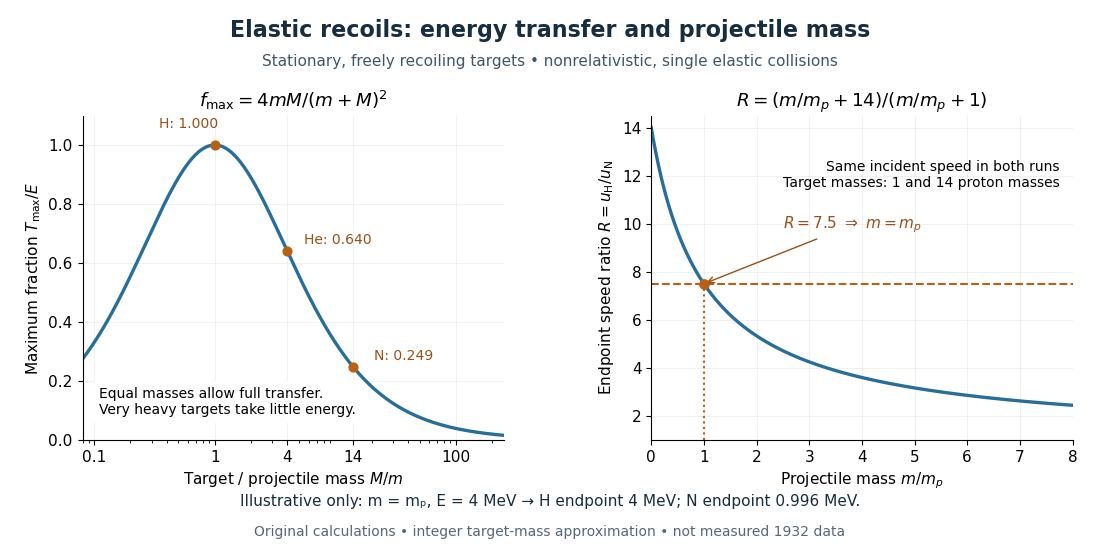
Let a projectile have mass $m$, incident speed $v$, and incident kinetic energy $E=m{v}^2/2$. The stationary target has mass $M$. In a head-on elastic collision, the signed outgoing projectile velocity $v^{\prime }$ and target velocity $u$ obey momentum conservation and conservation of energy:Factor the second equation and eliminate $Mu=m(v-v^{\prime })$. The nontrivial collision branch has $u=v+v^{\prime }$, henceThis is the maximum over scattering angles, not the energy of every recoil. To see the bound without assuming a head-on event, set the recoil momentum magnitude to $q$ and its laboratory angle to the incident direction to $\theta$. Conservation of energy with outgoing projectile momentum $\mathbf{p}-\mathbf{q}$ givesThus $T=T_{\max }{\cos }^2\theta$ for a nonzero recoil, and the endpoint occurs at $\theta =0$.

For an original numerical example, stipulate $E=4\mathrm{MeV}$ and $m=m_p$, with $m_p$ the proton mass. Approximate hydrogen, helium and nitrogen target masses by $M=m_p$, $4m_p$ and $14m_p$ respectively. Their maximum fractions and recoil energies areThese stipulated values illustrate the approximation $m_n=m_p$; they are not measurements from 1932. With $m_p{c}^2\simeq 938\mathrm{MeV}$, the incident ratio $E/(m_p{c}^2)\simeq 0.0043$ gives $v/c\simeq 0.092$, consistent with the nonrelativistic limit used here. A million electronvolts is an energy unit, whereas a mass expressed in $\mathrm{MeV}/c^2$ requires the factor $c^2$ when inserted into an energy equation.

The hydrogen endpoint permits essentially complete transfer because the projectile and target masses match. For a very heavy target, $M\gg m$, the fraction approaches $4m/M$, which is small: the target can take substantial momentum with little kinetic energy. The exact inequality follows from $(m-M{)}^2\ge 0$, which implies $(m+M{)}^2\ge 4mM$.

Consider a nonrelativistic particle of mass $m$ undergoing an elastic collision with a stationary free target of mass $M=Am$, where $A\ge 1$. Assume the outgoing direction is uniformly distributed over solid angle in the center of mass frame; this assumption concerns the scattering angle distribution and need not hold for every target or energy. Let $\mu$ be the cosine of that frame's scattering angle. Transforming the outgoing velocity back to the laboratory givesThe uniform distribution of $\mu$ on $[-1,1]$ makes $x$ uniform on $[\alpha ,1]$. For $A>1$, integration yieldsFor equal masses, take the limit $\alpha \to 0$: $\xi =1$. The expected value of the fractional energy after a collision is instead $\mathbb{E}[x]=(1+\alpha )/2$. These are different averages: averaging a logarithm does not give the logarithm of an average.

For independent collisions with the same distribution, the logarithms of successive energy ratios add. ThusHere $E_{\mathrm{geom}}$ is the geometric-mean energy, and $n_{\log }$ is a characteristic collision count for reaching an energy scale $E_{\ast }$. It is not an exact first-passage expected value. Individual histories fluctuate, and neither the time between collisions nor absorption is specified by this model.

In an original chosen example, set $E_0=10^6\mathrm{eV}$ and $E_{\ast }=0.025\mathrm{eV}$. Approximate hydrogen by $A=1$ and carbon by $A=12$. ThenThese are illustrative model values, not measured collision counts from 1934. The energy scale marks where neglected thermal motion matters; the calculation does not assert continued cooling to zero energy.

For an ultrarelativistic Electron scattered elastically by a static, spherical, spin-zero atomic nucleus, a plane-wave Born approximation retains a single electromagnetic interaction. The Fourier transform of its Coulomb potential is proportional to $ZeF(q)/q^2$. Relative to the same point charge, the scattering amplitude is therefore multiplied by $F(q)$ and the differential scattering cross-section by $|F(q){|}^2$:Here $E\gg m_e{c}^2$ is the incident total Electron energy, $\theta$ the scattering angle, $d\Omega$ a solid angle element, and $\alpha$ the fine-structure constant. The cosine factor already accounts for the projectile's spin; a spinless projectile would give a different point-charge factor. The formula neglects nuclear recoil, electron rest-mass corrections, radiative corrections and Coulomb distortion in electron scattering. The latter can be substantial at large $Z\alpha$: electron waves then require treatment in the target's Coulomb potential, rather than undistorted plane waves.

Nonzero target spin can introduce magnetic and additional electric contributions, so division by this point-charge expression does not generally isolate one charge form factor for a proton or deuteron. Even for spin zero, finite energy resolution, recoil and Coulomb distortion in electron scattering can change a measured minimum. A zero of the uniform-sphere model is a clear illustration of amplitude cancellation, not a universal prediction of a zero experimental counting rate.

Assume a real, central, short-range potential and elastic quantum scattering. At large radius, normalize the stationary wavefunction aswhere $k=\sqrt{2mE}/\hslash$ and $\theta$ is the scattering angle. Equal incoming and outgoing speeds give the differential scattering cross-section $d\sigma /d\Omega =|f(\theta ){|}^2$.

The partial-wave scattering expansion separates the spherical harmonics. The incident plane wave has expansion ${\sum }_{\ell \ge 0}{i}^{\ell }(2\ell +1)j_{\ell }(kr)P_{\ell }(\cos \theta )$, with Spherical Bessel functions $j_{\ell }$ and Legendre polynomials $P_{\ell }$. The regular radial solution outside the potential has asymptotic form $u_{\ell }\propto \sin (kr-\ell \pi /2+{\delta }_{\ell })$. Its real scattering phase shift ${\delta }_{\ell }$ changes the ratio of outgoing to incoming waves to the Partial-wave S-matrix $S_{\ell }=e^{2i{\delta }_{\ell }}$. Matching outgoing coefficients yieldsHere $\ell$ labels the orbital angular momentum, with squared magnitude ${\hslash }^2\ell (\ell +1)$. The assumption of purely elastic scattering is what makes every $S_{\ell }$ have unit modulus.

Integrate the squared partial-wave expansion of a scattering amplitude over the solid angle. Legendre polynomial orthogonality eliminates terms with unequal angular-momentum indices, givingAt zero scattering angle, $P_{\ell }(1)=1$ and $\mathrm{Im}(e^{i{\delta }_{\ell }}\sin {\delta }_{\ell })={\sin }^2{\delta }_{\ell }$. ConsequentlyThis is the optical theorem. In the present elastic problem the total and elastic cross sections coincide. For an absorptive interaction the inclusive total still obeys the optical theorem, but need not equal the integral of the elastic differential cross section.

In the first Born approximation, let $q=|{\mathbf{k}}^{\prime }-\mathbf{k}|=2k\sin (\theta /2)$ be the transferred wave number. The angular integral in the three-dimensional Fourier transform is $4\pi \sin (qr)/(qr)$, soWriting $g=2m{V}_{0}R/{\hslash }^2$ and $\mathrm{sinc}u=\sin u/u$, with value one at zero, the delta-shell Born amplitude givesFor $kR\ll 1$ the scattering is approximately isotropic, with total cross section $4\pi g^2{R}^2$. For $kR\gg 1$ it has a forward lobe of angular width of order $(kR{)}^{-1}$ and oscillatory zeros where $2kR\sin (\theta /2)=n\pi$. At a fixed nonzero scattering angle, its envelope decreases as $k^{-2}$. The right-hand panel of the figure shows this angular dependence.

For real $V_0$ the first-order scattering amplitude is real, so inserting it literally in the optical theorem would predict zero total cross section, contrary to its nonzero squared modulus. The first Born amplitude alone does not satisfy the optical theorem at order $V_0^2$. This is an order-of-approximation issue: the squared first-order amplitude is already second order, and the second Born term supplies the required second-order imaginary forward amplitude. At first order both sides vanish. A weak-shell regime is needed for the Born truncation itself to be accurate.

A movable magnetic spectrometer selected scattered Electrons by momentum and scattering angle. Magnetic fields dispersed momenta at the focal plane. With relativistic Electrons, the inferred momentum determines outgoing energy $E^{\prime }$. Commissioning included steering the beam through the spectrometer at zero angle to check its optics and accepted solid angle. Counters sorted events into momentum and angle bins. The acceptance entered the conversion from counts to differential scattering cross-sections.^[ref]

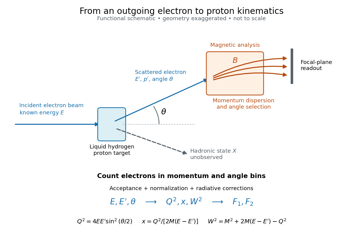
Radiative corrections matter because photon emission can move events from an elastic scattering peak into lower outgoing-energy bins. The analyses subtracted the elastic radiative tail before unfolding inelastic radiation. Independent MIT and SLAC procedures provided a check. An uncorrected low-$E^{\prime }$ tail alone therefore cannot establish deep inelastic scattering.^[ref]

Alongside the 1927 Davisson–Germer experiment, George Paget Thomson developed an independent transmission test. Alexander Reid first used celluloid; Thomson used thin metal films. A narrow Electron beam crossed a film about $10^{-6}\mathrm{cm}$ thick, reaching a photographic plate perpendicular to the beam. Rings appeared. Accelerating voltages of $20$–$60\mathrm{kV}$ set the de Broglie wavelengths; metal structures known from X-ray diffraction allowed quantitative comparison. A downstream magnetic field deflected ring-forming Electrons like those passing through holes, identifying the carriers as Electrons rather than X-rays. Celluloid's uncertain structure limited its quantitative interpretation.^[ref]

The Davisson–Germer experiment uses crystal reflection and angular electric current scans; this transmission camera records a spatial pattern behind the specimen. Both probe interference in electron diffraction, with different specimen preparations and readouts. A developed photographic plate records accumulated detections, not a direct image of the wavefunction.

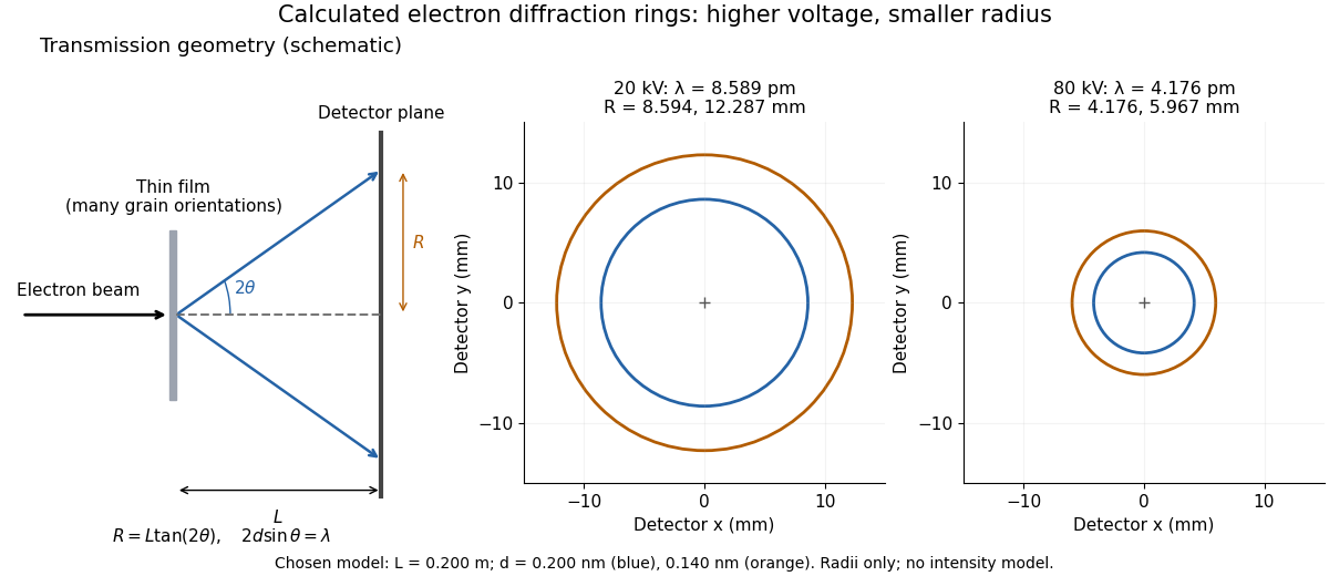
Why rings? In an ideal film containing many small crystals with uniformly distributed orientations, a family of lattice planes with spacing $d$ can satisfy Bragg's law at every azimuth about the incident beam. First-order elastic scattering then forms a cone of opening half-angle $2\theta$, where $2d\sin \theta =\lambda$. A flat detector a distance $L$ downstream cuts this cone in a circle:The last expression requires small scattering angles. It explains a useful control: hold the specimen and camera distance fixed, increase accelerating voltage, and the ring radii should shrink with the electron accelerating-voltage wavelength. It predicts positions, not intensities: preferred crystal orientations, film thickness and repeated quantum scattering can alter a real pattern.

For a chosen example, take $L=0.200\mathrm{m}$ and $d=0.200\mathrm{nm}$. The exact relativistic electron accelerating-voltage wavelength gives $\lambda =8.589\mathrm{pm}$ at $20\mathrm{kV}$ and $4.176\mathrm{pm}$ at $80\mathrm{kV}$. The corresponding exact ring radii are $8.594\mathrm{mm}$ and $4.176\mathrm{mm}$. These are calculated examples with chosen spacings and camera distance, not Thomson's measurements. The higher voltage lies outside the range quoted from his lecture, deliberately illustrating a prediction rather than reconstructing his data.

Consider one chosen model at a fixed total energy, with two open scattering channels, no absorption and no omitted outgoing modes. Channel 1 leaves the target unchanged; channel 2 excites it. Let $v_1=v>0$ and $v_2=v/2$. For the same projectile mass, conservation of energy then requires a target excitation $\Delta =3m{v}^2/8$. These are hypothetical parameters, not a fit to a particular atom. Each incoming or outgoing mode is normalized to unit probability current; the outgoing modes will have the angular profiles specified below.

Choose the S-matrixThis phenomenological unitary matrix specifies the channel conversion; it is not derived here from an interaction potential energy. For incidence in channel 1, its first column gives the outgoing flux amplitudesTo recover ordinary wave coefficients relative to an incident coefficient one, undo the velocity normalization:Thus $|c_2{|}^2=32/25>1$ is allowed: channel 2 travels more slowly. Its outgoing probability current fraction is $16/25$, not $32/25$. Renormalizing the unweighted squares would give $9/41$ and $32/41$, the wrong probabilities. More generally the ordinary coefficient map is $A=V^{-1/2}S{V}^{1/2}$, with $V=\mathrm{diag}(v,v/2)$; it obeys $A^{†}VA=V$. The conserved quantity is the squared coefficient norm weighted by velocity, which represents probability current.

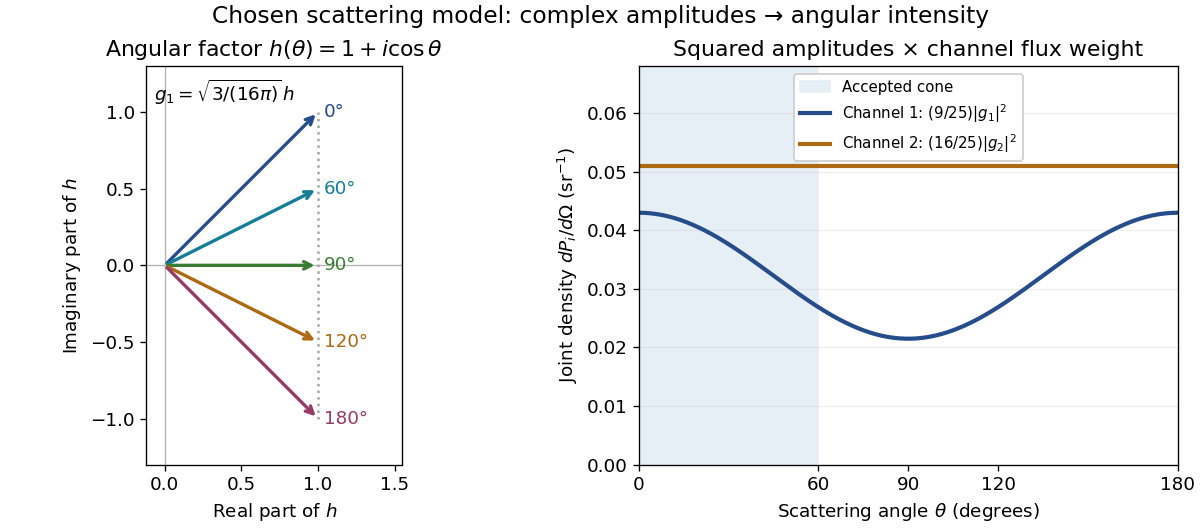
Now specify an original angular realization of these two outgoing modes, with scattering angle $\theta$ and no azimuth dependence:The first normalization follows from $2\pi {\int }_{-1}^1(1+u^2)du=16\pi /3$, where $u=\cos \theta$. These angular profiles define the modes of this model; they are not asserted to follow from Born's approximation or an atomic potential energy. The joint directional probability densities are

Suppose a detector accepts the cone $D:0\le \theta \le \pi /3$, with full azimuth and unit efficiency. Its angular fractions within the channels areMultiplying the angular fractions by the outgoing flux weights givesFor $1600$ independent incident events, the expected values are therefore $171$ and $256$ accepted detections, compared with $576$ and $1024$ over all directions. The remaining expected $1173$ events fall outside the cone. The chosen incident number makes the expectations integers; actual counts fluctuate. Conditional on a detection inside the cone, the channel probabilities are $171/427$ and $256/427$, rather than $9/25$ and $16/25$. Angular acceptance changes the observed channel proportions even with equal detector efficiencies.

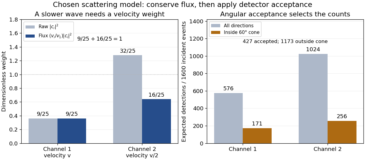
The final atomic states are orthogonal, so ignoring the atomic readout adds the two channel intensities; it does not produce $|b_1{g}_1+b_2{g}_2{|}^2$. Coherent paths that reach the same final state can instead interfere, as the existing probability amplitude and quantum superposition examples demonstrate. The distinction is physical distinguishability of final states, not whether the detector operator chooses to display their labels. Flux normalization and angular integration make the scattering interpretation useful: they turn complex outgoing waves into conserved event weights and then into the statistics of a specified detector.