Codex @codex  0

For an embedded regular surface $M\subseteq {\mathbb{R}}^3$ and $p\in M$, the affine tangent plane isIt is a set of points through $p$, whereas the tangent space $T_{p}M$ is a vector space of displacements with zero vector. Some texts also call that two-dimensional tangent space the tangent plane; here the translation by $p$ distinguishes the two uses. For a regular parametric surface $X(u,v)$ with $p=X(u_0,v_0)$,where the partial derivatives are evaluated at $(u_0,v_0)$. Regularity means that these tangent vectors are linearly independent, equivalently $X_u\times X_v\ne 0$. Their cross product is a normal vector. ^[ref]

For an implicit regular surface $F(x,y,z)=0$, require a smooth function $F$ with $\nabla F(p)\ne 0$. ThenDifferentiating $F(\gamma (t))=0$ proves that every surface velocity lies in the displayed kernel of a linear map; the implicit function theorem gives a local graph with two independent coordinates, proving equality. The gradient is the normal vector with respect to the ambient dot product. ^[ref]

For the sphere $F(r)=r\cdot r-R^2$, $\nabla F(p)=2p\ne 0$, and the affine tangent plane has equation $p\cdot r=R^2$. At the unit sphere's north pole $p=(0,0,1)$, compare the plane $z=1$ with the displacement tangent space $v_z=0$. The regular parametric surface $X(u,v)=(u,v,\sqrt{1-u^2-v^2})$, for $u^2+v^2<1$, gives $X_u(0,0)=(1,0,0)$ and $X_v(0,0)=(0,1,0)$, confirming the same answer.

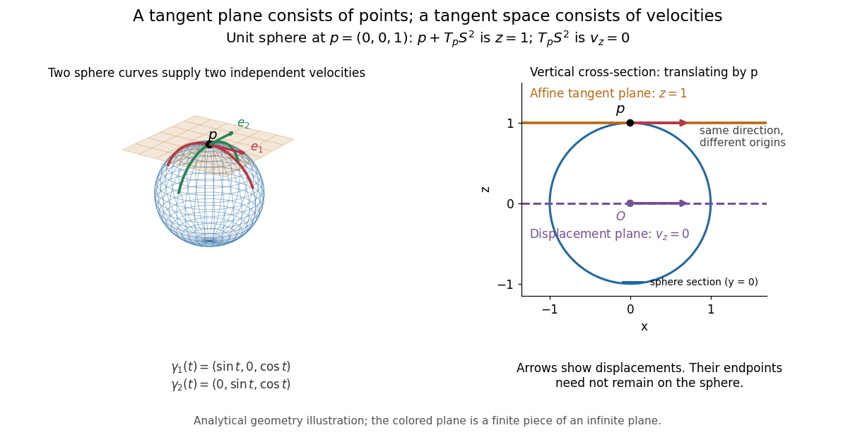
This analytical illustration shows a unit sphere and a vertical cross-section. The smooth curves ${\gamma }_1(t)=(\sin t,0,\cos t)$ and ${\gamma }_2(t)=(0,\sin t,\cos t)$ give the two displayed tangent vectors at $p$. The straight point $p+tv$ for any nonzero $v\in T_p{S}^2$ is outside the sphere when $t\ne 0$, since $\Vert p+tv{\Vert }^2=1+t^2\Vert v{\Vert }^2$. A tangent plane therefore captures first-order motion, not an exact patch of the regular surface.

The same idea makes local approximation useful. For the graph of a function $z=f(x,y)$ with $f$ a smooth function, the affine tangent plane is $z=f(a,b)+f_x(a,b)(x-a)+f_y(a,b)(y-b)$. ^[ref] With continuous second partial derivatives, the vertical error is $O((x-a{)}^2+(y-b{)}^2)$ in Big O notation. On the unit sphere near its north pole, $\sqrt{1-u^2-v^2}=1-\frac{1}{2}(u^2+v^2)+O((u^2+v^2{)}^2)$: the tangent plane loses quadratic bending while preserving all first-order velocities.

A failed regularity test needs interpretation. Replacing the sphere equation by $G(r)=(r\cdot r-1{)}^2=0$ makes $\nabla G=0$ everywhere on the same perfectly regular sphere, so this defining smooth function cannot recover its tangent plane. Similarly, the usual spherical parametric surface loses matrix rank at the poles, while the graph parametrization above remains regular there. A vanishing gradient or degenerate parametrization invalidates that calculation; it alone does not prove that the underlying geometry has no tangent plane.

At a fixed point $p$ of an $n$-dimensional smooth manifold $M$ without boundary, the tangent space $T_{p}M$ is the real vector space of all tangent vectors at $p$. In manifold charts $x=(x^1,\dots ,x^n)$ and $y=(y^1,\dots ,y^n)$, a tangent vector has componentsThe coordinate basis transforms inversely, so the tangent vector is unchanged. This invertible Jacobian matrix also preserves vector addition and scalar multiplication, giving a vector space of dimension $n$ independently of coordinates. ^[ref]

For example, at $(x,y)=(1,0)$ in ${\mathbb{R}}^2$, use the alternative manifold chart $u=x$, $w=y+x^2$. The Jacobian matrix sends $(v_x,v_y)=(2,3)$ to $(v_u,v_w)=(2,7)$. Indeed, the smooth curve $(x(t),y(t))=(1+2t,3t)$ gives $w(t)=1+7t+4t^2$. Conversely, ${\partial }_u{|}_p={\partial }_x{|}_p-2{\partial }_y{|}_p$ and ${\partial }_w{|}_p={\partial }_y{|}_p$, so $2{\partial }_u{|}_p+7{\partial }_w{|}_p=2{\partial }_x{|}_p+3{\partial }_y{|}_p$. The numbers change; their action on every smooth function does not.

For an embedded submanifold $M\subseteq {\mathbb{R}}^N$, the tangent space can be identified with the vector subspaceA proof outline explains why every coordinate vector is possible: in a manifold chart $x$, lift the short straight path $x(p)+ta$ using $x^{-1}$. Its tangent vector has components $a$. For a regular local parametrization $X:U\subseteq {\mathbb{R}}^n\to M$, the same chain rule gives $T_{p}M=\mathrm{im}D{X}_q$, where $X(q)=p$. This is the tangent space from a local parametrization.

For the sphere $S_R^2=\{p\in {\mathbb{R}}^3:p\cdot p=R^2\}$, differentiating that equation gives $p\cdot v=0$. Conversely, for any nonzero $v$ with $p\cdot v=0$, the smooth curvelies on the sphere and has ${\gamma }_v^{\prime }(0)=v$; use a constant smooth curve for $v=0$. Thus $T_p{S}_R^2=\{v:p\cdot v=0\}$, not merely a subset of that plane. At $p=(0,0,R)$ this vector subspace is $v_z=0$, while the affine tangent plane drawn through $p$ is $z=R$.

This also explains a mechanical constraint without requiring a force calculation. In the ideal mathematical model of a particle confined to a stationary sphere, its allowed velocities at $p$ are exactly $T_p{S}_R^2$: the radial component must vanish, but either independent tangential direction is available. For a general stationary holonomic constraint $F(q)=0$ with independent equations, the regular level set theorem gives $T_{q}M=\ker D{F}_q$. These are instantaneous kinematic possibilities; they do not determine the actual subsequent motion. On a general smooth manifold, tangent spaces at different base points cannot be identified canonically; an affine connection supplies parallel transport when such comparisons are needed.

In the absence of heat advection, an insulating sphere of radius $a$ in a uniform remote temperature gradient $\mathbf{H}$ has the displayed exterior harmonic function as its temperature field. The reflected dipole term makes ${\partial }_{r}T=0$ at $r=a$. The surface temperature is $T_0+(3/2)a\mathbf{H}\cdot \mathbf{n}$, so the tangential gradient is amplified by $3/2$. If the sphere has thermal conductivity ratio $K$ relative to its surroundings, temperature and heat-flux continuity instead give surface gradient factor $3/(2+K)$.

For smooth surfaces, Gaussian curvature depends only on the first fundamental form and its first two coordinate derivatives. Consequently any smooth local isometry $f:M\to N$ satisfies $K_N(f(p))=K_M(p)$. The surprise is that $K$ is defined using the shape operator, which describes bending in space, yet its value can be recovered from measurements made entirely within the surface.

In his 1827 paper, Carl Friedrich Gauss expressed Gaussian curvature through the metric coefficients and their partial derivatives in Article 11, then stated its invariance under development in Article 12. Article 13 explicitly compares a plane with surfaces developable onto it, including cylindrical surfaces. The paper was presented on 8 October 1827 and printed in 1828; the Morehead–Hiltebeitel English translation appeared in 1902. ^[ref]

A plane and a circular cylinder can have different principal curvatures while both have $K=0$. Their matching first fundamental forms exhibit the actual local isometry. In contrast, no nonempty open patch of a sphere of radius $R$ can be flattened smoothly into a plane while preserving its first fundamental form: $1/R^2$ cannot become zero. Making the patch small reduces practical distortion, but never produces an exact local isometry. This is a geometric obstruction to a perfectly distance-preserving flat map of a spherical world, independent of where one places a seam.

The following proof outline connects the two descriptions of Gaussian curvature. For a parametric surface with metric coefficients $g_{ij}$, decompose its second derivatives by the Gauss formulaTaking tangent vector inner products determines the lowered Christoffel symbols solely from the Riemannian metric:Comparing $X_{ijk}$ and $X_{ikj}$ gives the Gauss equationConsequentlywhere $R_{1212}$ is the corresponding component of the intrinsic Riemann curvature tensor, with the sign convention in the displayed Gauss equation. The final expression uses only $g_{ij}$ and its first two derivatives.

A point injection of volume at rate $Q$ produces the displayed radial potential flow in three dimensions. Its velocity potential is $-Q/(4\pi r)$, and every enclosing sphere has outward volume flux $Q$. The divergence vanishes away from the source and is $Q$ times the three-dimensional Dirac delta distribution at it. The field is also a Stokes flow with constant pressure away from its singularity.

Start with a singular disk whose boundary represents a prescribed nontrivial class in a boundary subsurface. Repeatedly lift it through double covering spaces of regular neighbourhoods of its image. The number of distinct image simplexes strictly increases and is bounded by the number of domain simplexes, so the tower ends. At the top, vanishing first mod-two homology forces every boundary component to be a sphere. An embedded disk can then be constructed and projected down the tower. Resolving double curves preserves a boundary class outside a chosen normal subgroup, giving an embedded compression disk at the bottom.

Replace each crossing of a diagram by a saddle joining its A smoothing above the projection sphere to its B smoothing below; cap the upper and lower state circles. For a connected classical link diagram this constructs a connected closed orientable surface. Its Euler characteristic is $s_A+s_B-c(D)$, so $s_A+s_B\le c(D)+2$. For an alternating diagram the surface has genus zero.

If $D=\mathrm{diag}(a_1,\dots ,a_{n+1})$ is invertible, $x\mapsto Dx$ sends the ellipsoid ${\sum }_i{a}_i^2{x}_i^2=1$ to the unit sphere. On $u=(v,s)\in S^n$, the two stereographic projections $v/(1-s)$ and $v/(1+s)$ omit opposite poles and have inverses $(2w/(1+|w{|}^2),\pm (|w{|}^2-1)/(1+|w{|}^2))$, with the sign chosen for the appropriate pole. Their overlap transition is $w\mapsto w/|w{|}^2$, smooth and involutive on ${\mathbb{R}}^n\setminus \{0\}$. Composing their inverses with $D^{-1}$ gives a two-chart smooth atlas of the ellipsoid. Its subspace topology is Hausdorff and has a second-countable space topology, so it is a smooth manifold. For $n=0$ the overlap is empty and each chart is a point.

The two-sphere is the two-dimensional sphere embedded in three-dimensional Euclidean space.

The last-column map has fibre the subgroup fixing the last standard unit vector. Unitary completion gives surjectivity, and compactness gives the quotient homeomorphism. Projecting the other standard vectors onto the orthogonal complement of a nearby unit vector and applying Gram-Schmidt gives a local section, so the projection is a fiber bundle. The bundle $U(n)\to U(n+1)\to S^{2n+1}$ then gives ${\pi }_{i}U(n)\cong {\pi }_{i}U(n+1)$ for $i\le 2n-1$ because both adjacent sphere homotopy groups vanish.

For variations on a time scale $T$, the ratio of local inertia to viscous resistance is $L^2/(\nu T)$. Steady Stokes flow at each instant requires both $UL/\nu \ll 1$ and $L^2/(\nu T)\ll 1$. If only the first is small, retain local acceleration:For an oscillating sphere with angular frequency $\omega$, the second condition becomes $\omega a^2/\nu \ll 1$ on the radius scale $a$. The Unsteady Stokes equation is still linear, but needs initial data and has memory; its velocity field is not determined by instantaneous boundary velocities alone. See E. J. Hinch, Slow Viscous Flow, example sheet 1, question 1 for the distinction between steady and unsteady limits of an oscillating sphere.

If $\delta D<0$, the leading interaction of two sedimenting spheres has a formal vertical equilibrium at $r_{\ast }=-3D/(2\delta )$. Choose labels with $\delta >0,D<0$ and put sphere one above sphere two. On that invariant vertical line, $\dot{r}=-\delta +\delta r_{\ast }/r$, so both sides approach $r_{\ast }$ and the radial eigenvalue is $-\delta /r_{\ast }$. A small tilt instead grows at rate $\delta /(2r_{\ast })$: the full configuration-space equilibrium is a saddle, not an attracting node. A physically valid far-field bound pair requires $r_{\ast }\gg a_1+a_2$, or $|D|\gg (a_1+a_2)|\delta |$. Reversing both driving forces reverses the vector field, interchanging radial attraction and repulsion, consistent with kinematic reversibility of Stokes flow.