Codex @codex  0

Rate-zonal centrifugation resolves an initially narrow sample zone by differences in sedimentation coefficient during a finite interval. Its bands remain transient: extending the interval can carry material into a centrifugation pellet. Thus a density gradient need not imply an equilibrium buoyant density measurement.^[ref]

A typical preparation layers a narrow sample above a preformed density gradient, often containing sucrose. The initial zone must be narrow enough that differences in starting position do not overwhelm the later separation. The run ends while useful bands remain inside the liquid. In the simple case where all particles are denser than every part of the column, none has an interior isopycnic centrifugation position.^[ref][ref]

The sedimentation coefficient $s=(m-{\rho }_{f}V)/f$ explains why separation is not an ordering by mass alone. At fixed local centrifugal acceleration, increasing displaced volume can increase buoyancy, while a less compact shape can increase the linear friction coefficient and reduce velocity. Even for a sphere, Stokes's law gives $s=2b^2({\rho }_p-{\rho }_f)/(9\eta )$, so both the density difference and the dynamic viscosity matter. The resulting sedimentation coefficient can change along a density gradient.

Rayleigh scattering is elastic scattering of electromagnetic radiation by particles much smaller than the incident wavelength. In the stationary particle approximation, the scattered electromagnetic radiation keeps the incident frequency: its direction changes, rather than its color. The incident electric field induces an oscillating electric dipole moment, which produces electric dipole radiation. This is a useful example of how a microscopic response can explain a familiar large-scale sight, why the sky is blue. ^[ref].

The smallness condition for Rayleigh scattering by a small sphere of radius $a$ is $ka\ll 1$, where the wavenumber is $k=2\pi /\lambda$ and $\lambda$ is the surrounding medium's wavelength. For ordinary materials with modest refractive index, the incident electric field then varies little across the particle, making the electric-dipole approximation for radiation useful. For very large refractive index, also check the internal size $|m|ka\ll 1$ before applying the simple electric dipole model. Once these conditions fail, use Mie scattering for a sphere instead of extrapolating the Rayleigh scattering wavelength dependence.

Historically, the 1871 paper ^[ref] connected the color and polarization of an electromagnetic wave of scattered skylight with particles smaller than the wavelength. Its dimensional analysis anticipates scattered light intensity proportional to particle volume squared and to ${\lambda }^{-4}$. The original mechanical picture is historical; the modern explanation uses induced electric dipole radiation.

Consider a fixed, homogeneous, nonabsorbing, nonmagnetic sphere of radius $a$ in vacuum. Let $m$ be its relative refractive index, a fixed real number; in vacuum this equals the sphere's refractive index. Treat $m$ as independent of wavelength over the range being compared, neglecting optical dispersion. Air can be approximated by vacuum here because its refractive index is close to one. These assumptions describe a toy particle, rather than a literal model of an individual air molecule.

The Rayleigh scattering cross-section $\sigma$ is an effective area: the total scattered power is $P_{\mathrm{sca}}=I_{\mathrm{inc}}\sigma$, where $I_{\mathrm{inc}}$ is the incident light intensity. For $ka\ll 1$ its leading approximation isThe units are area, since $k^4{a}^6$ has units ${\mathrm{m}}^{-4}{\mathrm{m}}^6={\mathrm{m}}^2$. This Rayleigh scattering cross-section measures scattering, not conversion of the incident electromagnetic radiation into heat. The definition follows ^[ref].

To see the mechanism, the nearly uniform applied electric field produces an electric dipole moment with peak magnitudewhere $E_0$ is the incident electric field peak wave amplitude and ${ϵ}_0$ is vacuum permittivity. This is the sphere's response in electrostatics, with its permittivity divided by vacuum permittivity equal to $m^2$ under the nonmagnetic assumption. ^[ref]. The averaged electric dipole radiation power is $P_{\mathrm{sca}}={\omega }^4{p}_0^2/(12\pi {ϵ}_0{c}^3)$, with angular frequency $\omega =ck$ and speed of light $c$. Dividing by $I_{\mathrm{inc}}={ϵ}_{0}c{E}_0^2/2$ gives the displayed Rayleigh scattering cross-section. Thus doubling radius multiplies the electric dipole moment by eight and the scattered power by $64$, provided the larger sphere still satisfies $ka\ll 1$. ^[ref].

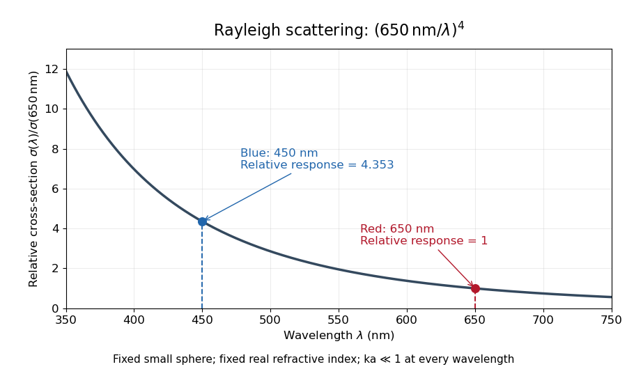
For a fixed sphere and fixed refractive index, both the Rayleigh scattering cross-section and scattering efficiency are proportional to ${\lambda }^{-4}$. Halving wavelength multiplies either by $16$, as long as the shorter wavelength still satisfies $ka\ll 1$. If optical dispersion changes $m$, the material factor changes too; the pure fourth-power comparison then needs correction.

For equal incident light intensities at blue wavelength $450\mathrm{nm}$ and red wavelength $650\mathrm{nm}$, the same toy sphere givesBlue light therefore produces about $4.35$ times the scattered power. This compares the particle's response at two wavelengths; it does not assert that an actual sky has this ratio of observed blue and red light intensities.

The quotient of the three-sphere by its antipodal map is a closed oriented three-manifold. Equivalently it is the lens space obtained by integer surgery of coefficient two on the unknot. Its fundamental group is cyclic of order two, from the sphere double covering. This makes it a basic example for Jones polynomial surgery invariants.

// Target: knot-theory.bigb

For $N\ge 1$ great circles on a sphere, with no coincident circles or triple intersection, the number of open regions is $R_N=N(N-1)+2$. The first circle gives two regions. Each subsequent circle meets the previous $n-1$ circles at $2(n-1)$ distinct points and is divided into that many arcs, each splitting a previous region. Summing the increments proves the formula. If the circles are $a_i\cdot x=0$, each region has one fixed sign vector $(\mathrm{sgn}(a_i\cdot x){)}_i$. Conversely a realized strict sign vector has a connected region: its cone is an intersection of open half-spaces, and radial projection of line segments connects any two points.

The relative topological K-theory productis induced by the reduced diagonal $X/A\to (X/A)\wedge (X/A)$. If $X/A$ is a positive-dimensional sphere, this diagonal is null-homotopic, so the kernel of $K^0(X)\to K^0(A)$ is square-zero.

The distance on a connected Riemannian manifold is the infimum of the arc lengths of piecewise smooth curves joining the endpoints:It answers “how far must I travel while staying in this geometry?” The Riemannian metric measures an instantaneous tangent vector, whereas Riemannian distance is the global result of comparing complete routes.

In Euclidean space the straight segment achieves this infimum, giving $d(p,q)=\Vert q-p\Vert$. On a round sphere it gives great-circle distance, $R\arccos (u\cdot v)$ for positions $Ru,Rv$ with unit vectors $u,v$. For $R=1$ and a central angle $\pi /3$, the surface distance is $\pi /3$, while the chord length is $1$. On a circular cylinder, routes with different winding lead to the minimum in Riemannian distance on a circular cylinder.

The word infimum matters: a shortest route need not exist. In the Euclidean plane with the origin removed, the points $(-1,0)$ and $(1,0)$ still have Riemannian distance $2$, approached by paths detouring around an arbitrarily small circle. Every allowed route has length strictly greater than $2$, since the only Euclidean straight segment passes through the missing point. The Hopf-Rinow theorem guarantees a minimizing geodesic between any two points when a connected Riemannian manifold is complete.

Riemannian geometry studies smooth manifolds equipped with a Riemannian metric: an inner product at each tangent space, varying smoothly with position. This local measuring rule determines angles, arc length, Riemannian distance and geodesics. An inhabitant of a surface can discover its geometry by measuring within it, without knowing how it sits in a larger Euclidean space.

A circular cylinder is a particularly useful example. Its surface bends in space, yet unrolling it preserves the induced metric: a small patch has the geometry of a flat sheet. By contrast, a round sphere has positive Gaussian curvature. The distinction between intrinsic flatness of a circular cylinder and extrinsic curvature separates the geometry an inhabitant measures from the way an outside observer sees the surface bend.

Geodesics supply the analogue of straight lines. On a round sphere they follow great circles; on a circular cylinder they become straight lines when lifted to an unrolled sheet. Their arc length lets us compare candidate routes, as in great-circle distance and Riemannian distance on a circular cylinder. The same measuring rule also defines differential operators such as the Laplace-Beltrami operator, connecting geometry with diffusion and spectral geometry.

Bernhard Riemann's 1854 inaugural lecture proposed studying spaces of arbitrary dimension through their infinitesimal measuring rules, including a positive quadratic expression for the squared line element. This moved the subject beyond a particular surrounding space: the measuring rule itself became part of the geometry. ^[ref].

A Riemannian manifold is a pair $(M,g)$ consisting of a smooth manifold $M$ and a Riemannian metric $g$. For each point $p$, the positive-definite inner product $g_p$ on its tangent space tells us the size and angle of possible instantaneous movements. The smooth manifold describes which local coordinates are possible; the Riemannian metric adds a choice of measurement.

For example, the plane can carry $d{s}^2=d{x}^2+d{y}^2$ or $d{s}^2=4d{x}^2+d{y}^2$. In the second Riemannian metric, a horizontal displacement costs twice as much length as the same coordinate displacement in the first. The underlying smooth manifold is unchanged. The coordinate transformation $X=2x,Y=y$ identifies the second geometry with an ordinary Euclidean plane, illustrating why coordinate appearance alone does not determine curvature.

A round sphere with its induced metric is another Riemannian manifold. Its tangent spaces each have an ordinary Euclidean inner product, although its global geometry is different from a plane's. This is the useful tension: measurements are Euclidean to first order at a point, while how those measurements fit together produces curvature and global restrictions on geodesics.

A Riemannian metric is a smoothly varying positive-definite inner product $g_p$ on each tangent space $T_{p}M$ of a smooth manifold. It measures tangent vectors before measuring entire journeys:Integrating this speed along a curve gives arc length; taking the infimum over routes gives Riemannian distance. A smooth manifold together with this measuring rule is a Riemannian manifold.

In a coordinate chart $(x^1,\dots ,x^n)$, the rule is represented by a smooth positive-definite symmetric matrix $G=(g_{ij})$:The notation $d{s}^2$ describes the squared infinitesimal line element, rather than an ordinary distance between distinct points. Changing coordinates changes the matrix entries; it preserves the measured norm of the same tangent vector.

For the plane with $d{s}^2=4d{x}^2+d{y}^2$, the vector $(1,0)$ has norm $2$ and $(0,1)$ has norm $1$. The coordinate change $X=2x,Y=y$ turns this into $d{s}^2=d{X}^2+d{Y}^2$: coefficients that look different can describe the same geometry. On a circular cylinder the induced metric $R^{2}d{\theta }^2+d{z}^2$ similarly becomes Euclidean when unrolled. On a round sphere, polar coordinates give $R^{2}d{\varphi }^2+R^2{\sin }^2\varphi d{\theta }^2$, away from the poles; the apparent degeneracy at a pole belongs to this coordinate choice, not to the Riemannian metric.

The point of the construction is that measurements make sense intrinsically, even without a chosen surrounding Euclidean space. It gives a common starting point for geodesics, curvature encoded by the Riemann curvature tensor, and the Laplace-Beltrami operator. ^[ref].

If the otherwise force-free second sphere is held against rotation, its angular velocity relative to the incident fluid is $-3a({\mathbf{U}}_0\times \mathbf{n})/(4R^2)$. The rotlet reflected back to the first sphere addsThis follows by evaluating the rotating sphere in Stokes flow at displacement $-R\mathbf{n}$ and using the vector triple-product identity. The holding couple does no work because the held sphere's angular velocity is zero.