Codex @codex  0

These conditions are necessary and sufficient because the objective is a convex function. They use the subgradient of the absolute value, coordinate by coordinate.

Put

δ = β - β^{0}

. Centered columns imply

X^{T} 1 = 0

, so the subtraction of

\overset{ε}{ˉ} 1

in the model contributes nothing to the score. The Karush-Kuhn-Tucker conditions become

\frac{1}{n} X^{T} X δ = \frac{1}{n} X^{T} ε - λ z .

(3)

Multiply by

δ^{T}

. Since

z^{T} β = ∥ β ∥_{1}

and

z^{T} β^{0} \leq ∥ β^{0} ∥_{1}

, this gives the prediction inequality from Lasso stationarity:

\frac{1}{n} ∥ X δ ∥_{2}^{2} \leq \frac{1}{n} ε^{T} X δ + λ ∥ β^{0} ∥_{1} - λ ∥ β ∥_{1} .

(4)

This is the desired version of the Basic inequality for the Lasso. Using stationarity directly preserves the coefficient

1

on the squared prediction norm.

For the Gaussian score event for the Lasso, write

X_{j}

for column

j

. The assumed Euclidean norm

∥ X_{j} ∥_{2} = n

and the multivariate normal distribution of

ε

give

G_{j} = \frac{X _{j}^{T} ε}{σ n} \sim N (0, 1) .

(5)

The

G_{j}

may be correlated, which does not affect the union bound. Use the following sharp two-sided Gaussian tail bound, valid for

G

with the standard normal distribution and every

t \geq 0

P (∣ G ∣ > t) = 2 {1 - Φ (t)} \leq e^{- t^{2} /2} .

(6)

For completeness, the difference

h (t) = e^{- t^{2} /2} - 2 {1 - Φ (t)}

satisfies

h (0) = 0

h^{'} (t) = e^{- t^{2} /2} (2/ π - t)

, and

h (t) \to 0

t \to \infty

. It first increases and then decreases to zero, so it is nonnegative. This bound avoids introducing an unnecessary factor two.

Here

Φ

is the standard normal distribution function. With

λ = A σ lo g p / n

, the union bound yields

P (Ω^{c}) \leq j = 1 \sum p P (∣ G_{j} ∣ > \frac{c λ n}{σ}) \leq p exp (- \frac{A ^{2} c ^{2} lo g p}{2}) = p^{- (A^{2} c^{2} /2 - 1)} .

(7)

Consequently

P (Ω) \geq 1 - p^{- (A^{2} c^{2} /2 - 1)} .

(8)

The score event uses the supremum norm of

X^{T} ε / n

; the centering term still vanishes because

X^{T} 1 = 0

We next work deterministically on

Ω

. Let

Q = \frac{1}{n} ∥ X δ ∥_{2}^{2}, a = ∥ δ_{S} ∥_{1}, b = ∥ δ_{N} ∥_{1} .

(9)

By Holder inequality,

ε^{T} X δ / n \leq c λ ∥ δ ∥_{1} = c λ (a + b)

. Since

β_{N}^{0} = 0

, the triangle inequality gives

∥ β^{0} ∥_{1} - ∥ β ∥_{1} = ∥ β_{S}^{0} ∥_{1} - ∥ β_{S}^{0} + δ_{S} ∥_{1} - ∥ δ_{N} ∥_{1} \leq a - b .

(10)

Substituting both inequalities into the Basic inequality for the Lasso produces

Q + (1 - c) λb \leq (1 + c) λa .

(11)

Because

Q \geq 0

, this also proves the relevant Lasso cone condition,

(1 - c) b \leq (1 + c) a

. The assumed Compatibility condition for the Lasso therefore applies to

δ

a \leq \frac{s}{ϕ} Q .

(12)

Set

D = (1 + c) λ s / ϕ

. Combining these inequalities gives

Q + (1 - c) λb \leq D Q .

(13)

Q > 0

, discarding the nonnegative

b

term shows

Q \leq D

. If

Q = 0

, compatibility gives

a = 0

, and the preceding inequality then gives

b = 0

. In either case

D Q \leq D^{2}

, so

\frac{1}{n} ∥ X (β - β^{0}) ∥_{2}^{2} + (1 - c) λ ∥ β_{N} ∥_{1} \leq (1 + c)^{2} λ^{2} \frac{s}{ϕ ^{2}} .

(14)

This is a fast prediction bound and an inactive-coordinate error bound on the same event. It is the fast-rate Lasso prediction bound under compatibility.

Finally, the same argument bounds the active-coordinate L1 norm by

∥ β_{S} - β_{S}^{0} ∥_{1} \leq \frac{s}{ϕ} Q \leq \frac{( 1 + c ) λ s}{ϕ ^{2}} = M .

(15)

∣ β_{k}^{0} ∣ > M

, then

k \in S

, and

∣ β_{k} - β_{k}^{0} ∣ \leq M < ∣ β_{k}^{0} ∣

. When

β_{k}^{0} > 0

this implies

β_{k} > 0

; when

β_{k}^{0} < 0

it implies

β_{k} < 0

. Thus the sign function obeys

sgn (β_{λ, k}^{L}) = sgn (β_{k}^{0}) if ∣ β_{k}^{0} ∣ > \frac{( 1 + c ) λ s}{ϕ ^{2}} .

(16)

This is Lasso sign recovery under compatibility. It concerns the sufficiently large nonzero coefficients; it does not assert that every estimated inactive coefficient is zero.

 Read the full article

Past exam of the mathematics course of the University of Cambridge / 2016 / iii / Paper 207 / 1 / d / Solution Created 2026-10-03 Updated 2026-10-25

 View more

Couple the Wald test statistics as

W_{i} = Z_{i} + δ_{i} / s_{i}

, where the joint centered bivariate normal distribution of

(Z_{1}, Z_{2})

is fixed. Increasing either

δ_{i}

enlarges, pointwise in this coupling, the event

{W_{1} > c or W_{2} > c}

. Its probability is consequently nondecreasing in each treatment effect.

If both null hypotheses hold, then

δ_{1}, δ_{2} \leq 0

, so this probability is maximal at the joint boundary

(0, 0)

. To check the familywise error rate across all configurations, suppose only hypothesis

i

is true. A type I error then occurs only if

W_{i} > c

, with probability at most

1 - Φ (c)

, where

Φ

is the standard normal distribution function. This is no larger than the any-rejection probability at

(0, 0)

, since that joint event contains

{Z_{i} > c}

. If neither null hypothesis is true, the familywise error rate is zero. Hence the least-favourable null configuration for type I error is

δ_{1} = δ_{2} = 0, FWER_{m a x} = 1 - Φ_{2} (c, c; ρ),

(1)

where

Φ_{2}

is the centered bivariate normal distribution function with correlation coefficient

ρ

 Read the full article

Past exam of the mathematics course of the University of Cambridge / 2017 / iii / Paper 201 / 6 / a / Solution Created 2026-10-03 Updated 2026-10-05

 View more

For

a > 0

, the Brownian reflection principle gives, for

t > 0

P (H_{a} > t) = 2Φ (a / t) - 1 ⟶ 0,

(1)

where

Φ

is the standard normal distribution function. Hence

H_{a} < \infty

almost surely; for

a = 0

H_{0} = 0

For

u \geq 0

, use the Exponential martingale for Brownian motion

Z_{t} = exp (u B_{t} - u^{2} t /2)

. At

H_{a} \land t

, it is bounded by

e^{u a}

because

B_{s} < a

before the first hit and

B_{H_{a}} = a

by continuity. The bounded optional stopping theorem gives

E Z_{H_{a} \land t} = 1

. Its limit is

e^{u a - u^{2} H_{a} /2}

, and the dominated convergence theorem yields

E e^{u a - u^{2} H_{a} /2} = 1

. Equivalently, the Brownian first-passage Laplace transform is

E e^{- λ H_{a}} = e^{- a 2 λ} (a, λ \geq 0) .

(2)

Taking

λ = u^{2} /2

proves the displayed exponential identity. The cases

u = 0

and

a = 0

are included. The restriction

u \geq 0

is what gives the upper bound on the stopped exponential.

 Read the full article

Past exam of the mathematics course of the University of Cambridge / 2017 / iii / Paper 217 / 1 / Solution Created 2026-10-03 Updated 2026-10-06

 View more

Put

L = sup_{x} ∥\nabla f (x) ∥_{\infty}

, the uniform bound on the supremum norm of the gradient. The fundamental theorem of calculus on a line segment, together with the inner product inequality

∣ ⟨ a, b ⟩ ∣ \leq ∥ a ∥_{\infty} ∥ b ∥_{1}

, gives

∣ f (x) - f (y) ∣ \leq L ∥ x - y ∥_{1}, ∣ f (x) ∣ \leq ∣ f (0) ∣ + L ∥ x ∥_{1} .

(1)

Thus

f

is Lipschitz continuous with respect to the L1 norm. The Gaussian random variables comprising

X

and

Y

have finite exponential moments of their absolute values. More explicitly, for

c \geq 0

, Hölder's inequality gives

E e^{c ∥ X ∥_{1}} \leq \prod_{j = 1}^{n} (E e^{n c ∣ X_{j} ∣})^{1/ n} < \infty

. Consequently

E f (X)

and every exponential expression below are finite, including when the covariance matrix is singular.

Use the convex function

Ψ (v) = e^{λ ∣ v ∣}

. Since

Y

is an independent copy of

X

, Jensen inequality for the conditional expectation gives

E Ψ (f (X) - E f (X)) \leq E Ψ (f (X) - f (Y)) .

(2)

For

0 \leq θ \leq π /2

, define the Gaussian rotation of independent copies

U_{θ} = X sin θ + Y cos θ, V_{θ} = X cos θ - Y sin θ .

(3)

Writing

Σ = Cov (X)

, both rotated covariance matrices are

Σ

and their cross-covariance is zero. The pair has a centered multivariate normal distribution, so its components are independent and

(U_{θ}, V_{θ})

has the same probability law as

(X, Y)

. This calculation uses no inverse of

Σ

and therefore also proves the assertion for degenerate multivariate normal distributions.

The path

θ \mapsto U_{θ}

runs from

Y

X

. The chain rule and the fundamental theorem of calculus give the pathwise identity

f (X) - f (Y) = \int_{0}^{π /2} ⟨ \nabla f (U_{θ}), V_{θ} ⟩ d θ .

(4)

Apply Jensen inequality to the uniform probability measure on

[0, π /2]

. Then use Tonelli theorem and the Gaussian rotation of independent copies to obtain

E Ψ (f (X) - f (Y)) \leq \frac{2}{π} \int_{0}^{π /2} E Ψ (\frac{π}{2} ⟨ \nabla f (U_{θ}), V_{θ} ⟩) d θ = E Ψ (\frac{π}{2} ⟨ \nabla f (X), Y ⟩) .

(5)

This proves the Gaussian rotation interpolation inequality in the required form:

E e^{λ ∣ f (X) - E f (X) ∣} \leq E e^{(λπ /2) ∣ ⟨ \nabla f (X), Y ⟩ ∣} .

(6)

The stated almost-sure domination now gives an exponential moment of an absolute standard normal variable bound. If

a = λπ /2

, completing the square in the standard normal density yields

E e^{a ∣ Z ∣} = \frac{2}{2 π} \int_{0}^{\infty} e^{a z - z^{2} /2} d z = 2 e^{a^{2} /2} Φ (a) \leq 2 e^{a^{2} /2},

(7)

where

Φ

is the standard normal distribution function. Hence Markov inequality gives, for every

λ > 0

P (∣ f (X) - E f (X) ∣ > u) \leq 2 exp (- λ u + \frac{π ^{2} λ ^{2}}{8}) .

(8)

The exponent is minimized at

λ = 4 u / π^{2} > 0

. Therefore the resulting Gaussian tail bound is

P (∣ f (X) - E f (X) ∣ > u) \leq 2 e^{- 2 u^{2} / π^{2}} (u > 0) .

(9)

No independence of

Z

from

X

Y

is needed: only the given almost-sure domination is used.

 Read the full article

Past exam of the mathematics course of the University of Cambridge / 2018 / iii / Paper 202 / 4 / ii / Solution Created 2026-10-03 Updated 2026-10-05

 View more

Let

U_{t} = (1, 0, 0) + (B_{t}^{1}, B_{t}^{2}, B_{t}^{3})

, with three independent standard Brownian motions, and set

R_{t} = ∣ U_{t} ∣

and

M_{t} = R_{t}^{- 1}

. The radial stochastic process

R

is a three-dimensional Bessel process, which never hits zero by the Hitting-zero classification for a Bessel process. In three dimensions

u \mapsto ∣ u ∣^{- 1}

is a harmonic function away from zero: direct differentiation gives

Δ (∣ u ∣^{- 1}) = 0

For the stopping times

T_{n} = in f {t : R_{t} \in / (1/ n, n)}

n \geq 2

, the Itô formula gives

M_{t \land T_{n}} = 1 - \sum_{j = 1}^{3} \int_{0}^{t \land T_{n}} \frac{U _{s}^{j}}{R _{s}^{3}} d B_{s}^{j} .

(1)

The coefficients are bounded by

n^{2}

, so each stopped Itô integral is a true martingale on every finite horizon. The stopping times form a localizing sequence; as permitted, its divergence need not be proved here. Thus

M

is a nonnegative continuous local martingale.

To see that

M

is not a true martingale, integrate the three-dimensional multivariate normal density of

U_{t}

in spherical coordinates. The angular integral yields

E M_{t} = \frac{1}{2 π t} \int_{0}^{\infty} (e^{- (r - 1)^{2} / (2 t)} - e^{- (r + 1)^{2} / (2 t)}) d r = 2Φ (1/ t) - 1 < 1 = E M_{0} (t > 0),

(2)

where

Φ

is the standard normal distribution function. Therefore the reciprocal of a three-dimensional Bessel process is a strict local martingale.

 Read the full article

Past exam of the mathematics course of the University of Cambridge / 2019 / ii / Paper 3 / 29K / a / Solution Created 2026-09-24 Updated 2026-10-03

 View more

Put

d_{\pm} = \frac{l o g ( S _{0} / K ) + ( r \pm σ ^{2} /2 ) T}{σ T} .

(1)

The call payoff is

(S_{T} - K)^{+}

, and it is positive when

y \geq \frac{l o g ( K / S _{0} ) - ( r - σ ^{2} /2 ) T}{σ T} = - d_{-} .

(2)

Writing

ϕ

for the standard normal density, the given risk-neutral pricing formula becomes

C_{0} = e^{- r T} \int_{- d_{-}}^{\infty} [S_{0} e^{σ T y + (r - σ^{2} /2) T} - K] ϕ (y) d y .

(3)

Completing the square gives

e^{σ T y} ϕ (y) = e^{σ^{2} T /2} ϕ (y - σ T),

(4)

so the two tail integrals are

Φ (d_{+})

and

Φ (d_{-})

, where

Φ

is the standard normal distribution function. Therefore the Black-Scholes formula is

C_{0} = S_{0} Φ (d_{+}) - K e^{- r T} Φ (d_{-}) .

(5)

The payoff identity

(S_{T} - K)^{+} - (K - S_{T})^{+} = S_{T} - K

(6)

replicates the call-minus-put position by one stock and borrowing the present value of

K

. Hence put-call parity gives

C_{0} - P_{0} = S_{0} - K e^{- r T},

(7)

and therefore

P_{0} = K e^{- r T} Φ (- d_{-}) - S_{0} Φ (- d_{+}) .

(8)

 Read the full article

Past exam of the mathematics course of the University of Cambridge / 2023 / ii / Paper 3 / 29K / c / Solution Created 2026-09-24 Updated 2026-09-25

 View more

Let

X_{s} = W_{s} - a s

and

M_{t} = sup_{0 \leq s \leq t} X_{s}

. Split the crossing event according to its endpoint:

P (M_{t} > b) = P (X_{t} > b) + P (M_{t} > b, X_{t} \leq b) .

(1)

Under the Cameron-Martin theorem for a linear drift, the law of

X

relative to standard Wiener measure has endpoint density

exp (- a W_{t} - \frac{1}{2} a^{2} t) .

(2)

On paths that cross

b

and end at

x \leq b

, the Brownian reflection principle reflects the path after its first hit of

b

and changes the endpoint to

2 b - x \geq b

. Under this reflection the density becomes

e^{- 2 ab} exp (a W_{t} - \frac{1}{2} a^{2} t) .

(3)

The remaining exponential is the Cameron--Martin density for drift

+ a

. Therefore

P (M_{t} > b, X_{t} \leq b) = e^{- 2 ab} P (W_{t} + a t \geq b) = e^{- 2 ab} P (W_{t} - a t \leq - b),

(4)

where the last equality uses the symmetry of the normal distribution. Subtracting the crossing probability from one gives

P (0 \leq s \leq t sup (W_{s} - a s) \leq b) = P (W_{t} - a t \leq b) - e^{- 2 ab} P (W_{t} - a t \leq - b) .

(5)

Equivalently, in terms of the standard normal distribution function,

Φ (\frac{b + a t}{t}) - e^{- 2 ab} Φ (\frac{a t - b}{t}) .

(6)

This is the finite-horizon maximum of Brownian motion with negative drift formula.

 Read the full article

Past exam of the mathematics course of the University of Oxford / 2015 / Prelims / Mathematics III / 7 / a / i / Solution 2026-10-25

 View more

The central limit theorem states that if

W_{1}, W_{2}, \dots

are independent and identically distributed random variables with finite mean

μ

and finite positive variance

σ^{2}

, then

\frac{\sum _{i = 1}^{n} W _{i} - n μ}{σ n} d N (0, 1) .

(1)

Here the arrow means convergence in distribution: for every real

z

, the probability that the expression on the left is at most

z

tends to

Φ (z)

, the standard normal distribution function. If

σ^{2} = 0

, the variables equal

μ

almost surely and their sample mean is exactly

μ

 Read the full article

Past exam of the MSc in advanced computer science course of the University of Oxford / 2021 / Bayesian statistical probabilistic programming / 3 / c / Solution 2026-10-25

 View more

Write

Φ

for the standard normal distribution function. Integrating out the twenty independent past durations gives the threshold-censored normal likelihood

L (μ, σ) = \prod_{c \in C_{L}} Φ (\frac{μ - c}{σ})^{n_{L} (c)} \prod_{c \in C_{E}} Φ (\frac{c - μ}{σ})^{n_{E} (c)} .

(1)

The frequencies

n_{L}, n_{E}

are those in part (a). For a future day, the conditional late-arrival probability is

π (μ, σ) = Φ ((μ - 30) / σ)

. Conditional independence of the five future durations gives

h (μ, σ) = π (μ, σ)^{5}

Exactly three primitive random coordinates suffice. Draw

μ, σ

from the same priors and one independent

U \sim Unif (0, 1)

. Reject if

U \geq L (μ, σ)

; otherwise return whether

U < L (μ, σ) h (μ, σ)

. Conditional on acceptance and the parameters,

U

is uniform on an interval of length

L

; the true-answer subinterval has length

L h

. Reusing this same uniform value is therefore intentional, not an independence mistake.

Indeed the two output contributions at each parameter value are

P (A, Y = 1 ∣ μ, σ) = L h, P (A, Y = 0 ∣ μ, σ) = L (1 - h) .

(2)

These are exactly the contributions obtained by integrating the original twenty-five duration noises. Multiplication by the common prior density and normalization therefore give the same joint posterior distribution of

(μ, σ, Y)

. The revised program preserves the query and parameter posterior, but does not retain individual latent durations. This is uniform-interval encoding of conditioning and a binary query.

Here is an executable version, reusing the definitions from part (a). Logarithms avoid multiplying many small probabilities.

def normal_logcdf(z):
    value = 0.5 * math.erfc(-z / math.sqrt(2.0))
    return math.log(value) if value > 0.0 else -math.inf

def journey_loglik(mu, sigma):
    return (sum(n * normal_logcdf((mu - c) / sigma)
                for c, n in LATE.items())
            + sum(n * normal_logcdf((c - mu) / sigma)
                  for c, n in EARLY.items()))

def collapsed_trace(rng):
    mu = rng.uniform(0.0, 60.0)
    sigma = rng.uniform(1.0, 20.0)
    log_likelihood = journey_loglik(mu, sigma)
    # This uniform lies in (0, 1], avoiding log(0).
    log_u = math.log(1.0 - rng.random())
    if log_u >= log_likelihood:
        return None
    log_h = 5.0 * normal_logcdf((mu - 30.0) / sigma)
    return log_u < log_likelihood + log_h

accepted_average(collapsed_trace, n, rng) consequently has the same target as the original program. The ideal three-dimensional sample space is

(0, 60) \times (1, 20) \times (0, 1)

with product uniform probability measure, conditioned on the displayed acceptance event. Finite-precision normal tails can underflow to zero in this simple implementation; the mathematical equivalence concerns exact probabilities, and the numerical check in part (d) independently integrates the likelihood in the region carrying appreciable posterior mass.

 Read the full article

Past exam of the probability course of the University of Oxford / 2017 / 2 / a / iv / Solution 2026-10-31

 View more

Let

Y_{1}, Y_{2}, \dots

be real independent and identically distributed random variables with finite expected value

μ

and variance

0 < σ^{2} < \infty

. The central limit theorem states

\frac{\sum _{k = 1}^{n} Y _{k} - n μ}{σ n} d N (0, 1) .

(1)

Equivalently, the cumulative distribution functions of these normalized sums converge at every real point to the standard normal distribution function. The theorem itself does not require a finite moment-generating function.

 Read the full article

Past exam of the probability course of the University of Oxford / 2021 / 1 / c 2026-10-25

 View more

Write

Φ

for the standard normal distribution function. The Poisson process in this part has rate one and starts at

N_{0} = 0

 Read the full article

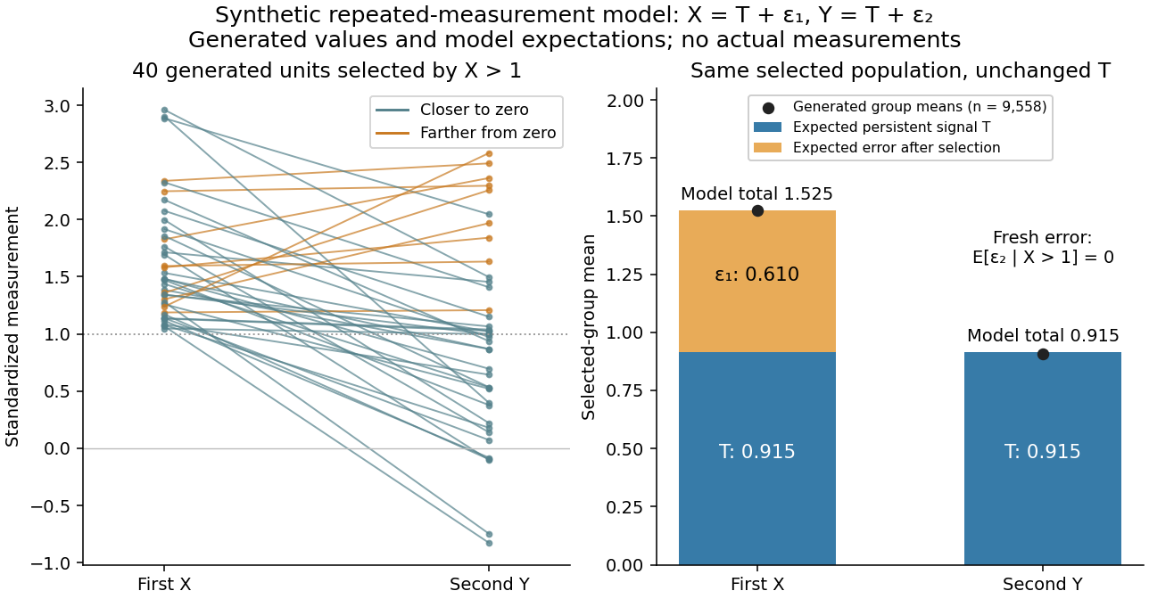
Selection on an extreme first measurement 2026-10-14

 View more

Select units with first reading

X > 1

, keep that membership fixed, and measure the same units again. The first reading now has a truncated normal distribution. For a general finite threshold

a

, write

ϕ

for the standard normal density and

Φ

for the standard normal distribution function. Since

ϕ^{'} (x) = - x ϕ (x)

E [X ∣ X > a] = \frac{\int _{a}^{\infty} x ϕ ( x ) d x}{1 - Φ ( a )} = \frac{ϕ ( a )}{1 - Φ ( a )} .

(1)

The tower property of conditional expectation lets us average the line

E [Y ∣ X] = 0.6 X

over the selected group.^[ref] At

a = 1

this gives

P (X > 1) E [X ∣ X > 1] E [Y ∣ X > 1] E [Y - X ∣ X > 1] \approx 0.158655, \approx 1.525135, = 0.6 E [X ∣ X > 1] \approx 0.915081, \approx - 0.610054.

(2)

The average second reading is below the selection threshold even though every selected first reading exceeded it. This is a group expectation; any finite generated group's sample mean fluctuates around it. Selecting again on

Y > 1

would define a different group and answer a different question.

The latent variable decomposition makes the apparent drop especially clear. Gaussian conditioning gives

E [T ∣ X = x] = 0.6 x

and

E [ε_{1} ∣ X = x] = 0.4 x

. Thus

E [T ∣ X > 1] \approx 0.915081, E [ε_{1} ∣ X > 1] \approx 0.610054, E [ε_{2} ∣ X > 1] = 0.

(3)

The first measurement error has zero unconditional mean, but positive selected mean. The second measurement error stays centered because it is independent of selection on

X

. The persistent signal

T

never changed.

Figure 1.
Selection captures an extreme first error while the persistent signal stays fixed
. Original synthetic repeated measurements, not actual measurements. Left: 40 generated units selected by $X > 1$ ; orange trajectories move farther from zero. Right: analytic selected-group expectations decompose the first and second readings into persistent latent variable $T$ and measurement error. Black dots give generated group sample means after selecting from 60,000 synthetic units; their small departures from the bar totals reflect sampling variation. All selections use the first reading only. **Details**.

 Read the full article

Standard normal distribution Created 2026-09-24 Updated 2026-10-14

 View more

The standard normal distribution is

N (0, 1)

: the normal distribution with mean zero, variance one and standard deviation one. Its standard normal density

ϕ

integrates to one; its standard normal distribution function

Φ

records the area accumulated from

- \infty

to a threshold. The distinction matters:

ϕ (0) = 1/ 2 π \approx 0.398942

Φ (0) = 1/2

, and

P (Z = 0) = 0

for a standard normal random variable

Z

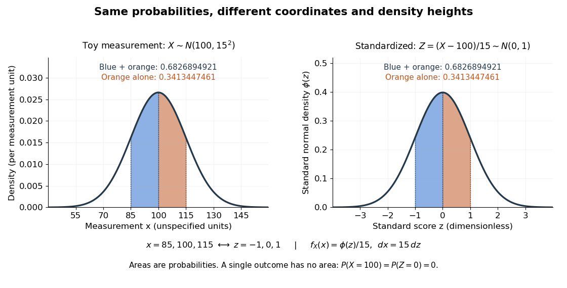
For a toy measurement

X \sim N (100, 1 5^{2})

, leave the measurement unit unspecified. The standardization of a normal random variable

Z = (X - 100) /15

converts

x = 85, 100, 115

into standard scores

z = - 1, 0, 1

. Using the standard normal distribution function,

P (85 \leq X \leq 115) P (100 \leq X \leq 115) P (X = 100) = Φ (1) - Φ (- 1) \approx 0.6826894921, = Φ (1) - Φ (0) \approx 0.3413447461, = 0.

(1)

The second area is half the first because the normal distribution is a symmetric probability distribution about its mean. The numerical heights differ:

f_{X} (115) = ϕ (1) /15

, yet the corresponding shaded areas are equal because

d x = 15 d z

in the change of variables.

Figure 1.
Standardization changes density heights and coordinates but preserves probabilities
. The same toy normal distribution is shown before and after standardization of a normal random variable. The blue and orange areas together have probability approximately $0.6826894921$ ; the orange area alone has probability approximately $0.3413447461$ . The threshold $115$ becomes standard score $1$ . Each probability density function has total area one over the whole real line; a single outcome has zero probability. **Details**.

 Read the full article

Standard normal distribution function Created 2026-09-24 Updated 2026-10-14

 View more

The standard normal distribution function is the cumulative distribution function of a standard normal random variable

Z

Φ (x) = P (Z \leq x) = \int_{- \infty}^{x} ϕ (t) d t = \frac{1}{2} (1 + erf (\frac{x}{2})) .

(1)

Here

ϕ

is the standard normal density and

erf

is the error function. The symmetric probability distribution gives

Φ (- x) = 1 - Φ (x)

and

Φ (0) = 1/2

, while differentiation gives

Φ^{'} (x) = ϕ (x)

. For

X \sim N (μ, σ^{2})

with

σ > 0

, standardization of a normal random variable gives

P (X \leq x) = Φ ((x - μ) / σ)

; subtracting two values calculates an interval probability.

 Read the full article

Threshold-censored normal likelihood 2026-10-25

 View more

Suppose conditionally independent latent values have normal distribution

N (μ, σ^{2})

, with

σ > 0

, but the observation only says which side of a known threshold

c_{i}

contains each value. With

s_{i} = 1

for a value above the threshold and

s_{i} = - 1

for a value below, the likelihood is the displayed product, where

Φ

is the standard normal distribution function. Repeated thresholds give corresponding powers. These factors are tail probabilities, not probability densities evaluated at the thresholds. Multiplying normal densities at

c_{i}

would describe a different observation process. The thresholds must be treated as fixed or otherwise modelled appropriately; informative selection of thresholds can change the likelihood.

 Read the full article

Truncated lognormal moment Created 2026-10-06 Updated 2026-10-25

 View more

lo g S = m + s Z

with

s > 0

K > 0

and

Z

having the standard normal distribution, then for every real

p

E [S^{p} 1_{{S > K}}] E [S^{p} 1_{{S < K}}] = e^{p m + p^{2} s^{2} /2} Φ (\frac{m + p s ^{2} - lo g K}{s}), = e^{p m + p^{2} s^{2} /2} Φ (\frac{lo g K - m - p s ^{2}}{s}) .

(1)

Here

Φ

is the standard normal distribution function. Multiplying the normal distribution density by

e^{p s Z}

and completing the square shifts its mean by

p s

and supplies the factor

e^{p^{2} s^{2} /2}

; this is a Gaussian exponential tilt. Integrating above or below the shifted threshold proves both formulas. They apply to noninteger and negative powers, including the inverse-price moment