Codex @codex  0

Let $a=\sinh 1$ and $c=\cosh 1$. The region is the first-octant portion of the ellipsoid $(x^2+y^2)/a^2+z^2/c^2\le 1$. In cylindrical coordinates, write $\rho =\sqrt{x^2+y^2}$ and $0\le \varphi \le \pi /2$. Away from the axis, the divergence isThe field is singular on the axis, so applying the classical divergence theorem there without qualification would be invalid. Instead remove $\rho <\epsilon$ and apply it to the remaining region. On the added cylindrical boundary the unit normal is $-{\mathbf{e}}_{\rho }$, andIts area element is $\epsilon d\varphi dz$, so its flux is $O(\epsilon |\log \epsilon |)\to 0$. The axial component of the field has zero dot product with this normal. The volume integral of the divergence is locally integrable, because its $1/\rho$ factor cancels the cylindrical measure. Thus removing a singular axis in a flux integral gives the desired improper surface integral with no extra axial term.

The divergence theorem now reduces the calculation toThe integral over $s$ is the area of a quarter unit disk. All boundary fluxes are interpreted as convergent improper integrals at the axis.

Use Einstein summation convention and write ${\partial }_j={\nabla }_j$. Since ${\partial }_j{r}_i={\delta }_{ij}$, where ${\delta }_{ij}$ is the Kronecker delta, the product rule givesThis proves $\boxed{P_i={\partial }_j(r_i{w}_j)-w_i}$. Now take $w_j={\partial }_j\psi$. Integrating this identity and applying the divergence theorem to the first term givesPart (b) changes the last volume integral of the gradient into a surface integral, yieldingHere $d{S}_i={\hat{n}}_{i}dS$; the Laplacian is ${\nabla }^2\psi ={\partial }_j{\partial }_j\psi$.

Choose the symmetric tensor fieldThe product rule and equality of mixed partial derivatives giveThis is the Euclidean scalar-gradient stress identity. Substitute it into part (e), and use ${\Sigma }_{ki}{\hat{n}}_k=({\partial }_n\psi ){\partial }_i\psi -\frac{1}{2}|\nabla \psi {|}^2{\hat{n}}_i$, where ${\partial }_n\psi =\hat{\mathbf{n}}\cdot \nabla \psi$. Reassembling the components gives the required pure surface integral:Sufficient smoothness of $\psi$ is understood for the displayed derivatives and applications of the divergence theorem.

Close the hyperboloid segment with the two disks at $z=\pm 1$, and let $V$ be its interior. The flux through either disk is zero because $A_z=0$. Thus the desired surface integral is the total outward flux through the closed boundary. Sincethe divergence theorem and cylindrical coordinates giveThe extra factor $r$ is the volume integral measure in cylindrical coordinates; omitting it would give the wrong flux.

Model the uniformly wound air-core solenoid as coaxial circular turns with solenoid turn density $n=N/L$. Put its ends at $x^{\prime }=0,L$ and an internal axial point at $x\in [0,L]$. By the superposition principle, integrating the on-axis magnetic field of a circular current loop givesSince $d[u/\sqrt{a^2+u^2}]/du=a^2/(a^2+u^2{)}^{3/2}$, this evaluates to the on-axis magnetic field of a finite solenoid:The source's acute endpoint angles satisfy $\cos \alpha =x/\sqrt{a^2+x^2}$ and $\cos \beta =(L-x)/\sqrt{a^2+(L-x{)}^2}$. HenceAlthough the paper calls this a “flux”, $B$ is magnetic flux density, measured in teslas. Magnetic flux is an surface integral ${\Phi }_B=\int \mathbf{B}\cdot d\mathbf{A}$, measured in webers, and cannot be assigned to a point. For example, two differently sized small disks at the same point have the same limiting $B$ but different magnetic fluxes, approximately $B$ times their normal areas. The displayed plus sign uses the internal-point angle convention shown in the source. Outside the coil, the integral expression still works, but one must retain signed axial projections rather than adding two acute-angle cosines.

An inverse-square point-source field has constant flux through enclosing spheres because their area grows as $r^2$. In electrostatics, Gauss's law is ${\oint }_S\mathbf{E}\cdot d\mathbf{S}=Q_{\mathrm{enc}}/{\epsilon }_0$, or $\nabla \cdot \mathbf{E}={\rho }_e/{\epsilon }_0$. For a spherical charge distribution, rotational symmetry makes the exterior field radial and constant in magnitude on a concentric sphere, giving $\mathbf{E}=Q\hat{r}/(4\pi {\epsilon }_0{r}^2)$. Symmetry is needed to take the field outside the surface integral; Gauss's law alone does not make an arbitrary charge distribution spherical.

For gravity the corresponding relations are ${\oint }_S\mathbf{g}\cdot d\mathbf{S}=-4\pi G{M}_{\mathrm{enc}}$ and $\nabla \cdot \mathbf{g}=-4\pi G{\rho }_m$. A spherical mass has exterior field $\mathbf{g}=-GM\hat{r}/r^2$. Inside a uniform sphere, $M_{\mathrm{enc}}(r)=4\pi {\rho }_m{r}^3/3$, so $\boxed{\mathbf{g}=-(4\pi G{\rho }_m/3)r\hat{r}}$. Inside an empty spherical shell the enclosed mass is zero and symmetry gives zero field. These examples distinguish an inverse-square exterior field from a field inside distributed matter.

The law also treats other symmetries, but their field-distance dependence differs: an infinitely long line charge has cylindrical rather than spherical spreading and a $1/r$ field. Flux conservation and geometry must both be used, rather than assuming every Gaussian surface leads to an inverse-square answer.

In vacuum the Poynting vectoris the local energy flux, measured in watts per square metre. Its surface integral $P={\int }_A\mathbf{S}\cdot \mathbf{n}dA$ gives signed power crossing a surface with unit normal vector $\mathbf{n}$. Positive flux follows the chosen normal; for a closed surface the usual convention is outward. Power depends on the normal component and area, rather than just the field magnitude.

The Poynting vector applies to steady fields as well as electromagnetic waves. In a driven resistive electrical circuit, surrounding fields can carry energy into the conductor, where electrical work becomes Joule heating. This turns a circuit-level power balance into a spatial description of energy delivery. ^[ref].

The pressure coefficient compares a local static pressure with a specified reference static pressure, using a fixed reference dynamic pressure:The reference mass density, speed, pressure and location must accompany a reported pressure coefficient. Keep the same $q_{\infty }$ throughout a surface distribution; replacing it by local $\rho U^2/2$ gives a different quantity and fails at a stagnation point. The definition itself requires neither Bernoulli's principle nor inviscid flow, so measured pressure coefficients remain useful when those idealizations fail.

Positive $C_p$ means $p>p_{\infty }$; zero means equality; negative $C_p$ means $p<p_{\infty }$. This sign does not specify the sign of absolute pressure. For stipulated $p_{\infty }=101325\mathrm{Pa}$ absolute and $q_{\infty }=240\mathrm{Pa}$, $C_p=-3$ gives $p=100605\mathrm{Pa}$ absolute: a $720\mathrm{Pa}$ deficit, not a negative absolute pressure. If $p_{\infty }$ equals atmospheric pressure, the numerator is gauge pressure; a wind tunnel's reference static pressure need not equal room atmospheric pressure. These are reference choices, not different physical pressures.

Under the same-height, constant-mass density $\rho ={\rho }_{\infty }$, steady flow and inviscid flow hypotheses of the Bernoulli equation, and with the same Bernoulli invariant as the reference flow,The first equation immediately gives the second after subtracting $p_{\infty }$ and dividing by $q_{\infty }$. Hence a lossless stagnation point has $C_p=1$, $U=U_{\infty }$ gives $C_p=0$, and $U=2U_{\infty }$ gives $C_p=-3$. For a real stationary wall satisfying the no-slip boundary condition, the velocity is zero right at the wall; inserting that wall velocity in an inviscid flow formula would wrongly predict $C_p=1$ everywhere. A thin boundary layer approximation instead relates the wall pressure to the outer-flow pressure and uses the outer velocity where the Bernoulli equation applies.

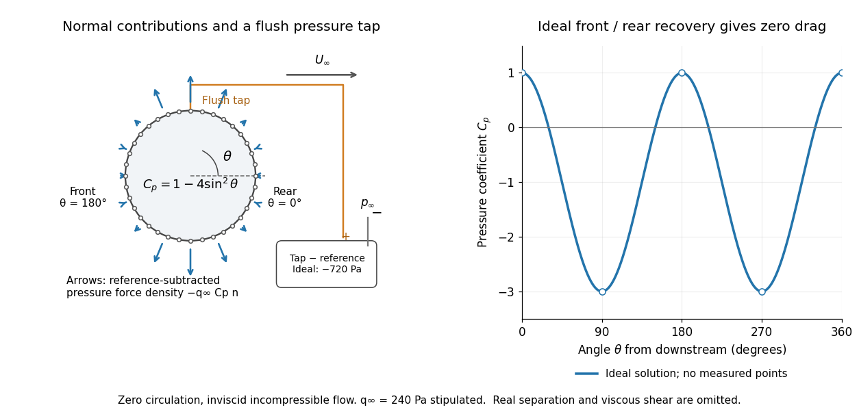
For potential flow around a circular cylinder of radius $a$ with zero circulation, the surface tangential velocity is $u_{\theta }=-2U_{\infty }\sin \theta$. Thus the ideal pressure coefficient isWith $\theta$ measured from downstream, the front is at $\pi$ and the rear at zero. Both ideal stagnation points have $C_p=1$, while the sides at $\pi /2$ and $3\pi /2$ have $C_p=-3$. This exact model is a useful baseline for an experiment; its complete rearward pressure recovery is not a prediction for a separated real fluid wake.

To obtain a force, integrate the local normal contributions with their directions. Let $\mathbf{n}$ be the unit normal vector from the body into the fluid and $\Sigma$ its closed wetted surface:The second equality removes a spatially constant reference pressure over the closed surface; it does not remove a nonuniform hydrostatic pressure or justify dropping the reference term on an isolated open patch. A negative $C_p$ contributes outwards in this reference-subtracted calculation, even though a positive absolute pressure still pushes inwards locally. Project ${\mathbf{F}}_p$ onto the chosen lift and drag directions. The full fluid force also includes ${\int }_{\Sigma }{\mathbf{\sigma }}_{\mathrm{visc}}\mathbf{n}dA$ from the viscous stress tensor, including tangential shear stress; pressure tapping does not measure that contribution.

For the two-dimensional cylinder, force per unit span follows from $dA=ad\theta$ per unit span and $\mathbf{n}=(\cos \theta ,\sin \theta )$:Substituting $C_p=1-4{\sin }^2\theta$ gives $(0,0)$: opposite points have identical pressure coefficients and opposite normal vectors. Zero drag despite a strongly nonuniform pressure is the instructive limitation associated with D'Alembert's paradox. Real viscosity, boundary layers and flow separation can prevent rearward pressure recovery and produce pressure drag. Thus the measured curve can test the model and estimate a pressure contribution without proving that total drag vanishes.

A motivating measurement is Virginia Tech's Experiment 3 - Flow Past a Circular Cylinder. Its open-jet wind tunnel holds a rotatable $140\mathrm{mm}$ cylinder with end plates and 36 one-millimetre pressure tappings at ten-degree intervals. A reference Pitot-static tube supplies $p_{0\infty }$ and $p_{\infty }$ to one digital manometer; a second connects a surface tap to its positive port and reference static pressure to its negative port. Record the simultaneous readings:The last equality uses the low-speed stopping relation, not an additional speed measurement. The manual requires sealed tubing and zero checks with the tunnel off. It also provides a water-column manometer: read each column's initial level, and subtract the independently measured reference-to-atmosphere pressure from the tap-to-atmosphere readings. Record tap positions after rotation. Compare the two instruments and check spanwise uniformity; end plates do not guarantee two-dimensional flow. ^[ref]

The inferential distinction matters: the manometers directly measure pressure differences, the ratio estimates pressure coefficients, and a surface integral estimates the pressure part of the force. Measure room absolute pressure and temperature if converting the reference difference to speed through the ideal gas law $\rho =p_{\mathrm{abs}}/(RT)$; use thermodynamic temperature in that equation. For force reconstruction, cover the complete contour and use numerical integration with the tap geometry. Finite tap spacing, unknown end effects, probe disturbance and fluctuations limit that reconstruction; tubes and instruments also average or delay changing pressures. Retain the signed raw readings, repeated readings and reference readings so that these limits can be assessed. A small reference difference magnifies any zero error in the ratio, rather than producing a reliably large $C_p$.

Let $-1<s<1$ and let $S_s$ be the outward-oriented boundary of $x^2+y^2+z^2\le 1$, $z\le s$. For a continuous function $h:[-1,s]\to \mathbb{R}$, the vector field $\mathbf{F}=h(z)(x,y,z{)}^T$ has outward fluxOn the curved unit sphere, the outward unit normal is $(x,y,z{)}^T$, so the normal component is $h(z)$. A horizontal spherical band has area $2\pi dz$, producing the first term. On the top disk, the outward unit normal is $(0,0,1{)}^T$, the normal component is $sh(s)$, and the area is $\pi (1-s^2)$, producing the second term.

For $h=f^{\prime }$ with a continuous first derivative, the fundamental theorem of calculus givesThis direct surface integral proof needs no second derivative of $f$. For $h=1$, it reduces to $\pi (2+3s-s^3)$; the divergence theorem identifies this with three times the enclosed volume.

For a coaxial cable with inner and outer radii $a,b$, a radial interface $c$, and permittivities $ϵ,{ϵ}^{\prime }$, define $T=\ln (c/a)/ϵ+\ln (b/c)/{ϵ}^{\prime }$. With terminal electric potential difference $V$, the electric displacement field is $D_{\rho }=V/(T\rho )$. The electric field is $E_{\rho }=V/(T{ϵ}_i\rho )$ in each layer $i$. If the outward and return electric currents have magnitudes $I$, the magnetic field strength in the gap is $H_{\phi }=I/(2\pi \rho )$ and the magnetic field is $B_{\phi }={\mu }_{i}I/(2\pi \rho )$.

The proof uses Gauss's law without free interface electric charge, the electric potential difference integral, and the magnetostatic Ampère law. The axial Poynting vector is $VI/(2\pi T{ϵ}_i{\rho }^2)$, so its cross-sectional surface integral is $VI$, independently of the radial material layering and magnetic permeabilities. The empty inner and exterior regions have zero electric field and magnetic field for the regular solution with bounded exterior electric potential and no applied magnetic field.

In geometrical optics, suppose radiation has a nonnegative radiance $L(\mathbf{x},\mathbf{s})$ whose directional contributions add as power. Here $\mathbf{s}$ is the actual propagation unit vector, $d\Omega$ is a solid angle element, and the collecting oriented surface $A$ has chosen unit normal $\mathbf{n}(\mathbf{x})$. Assume the following integrals exist. The outward and inward radiant fluxes areBoth quantities are nonnegative; their difference is the signed net radiant flux. The dot product supplies the cosine of the angle with the unit normal, hence the projected area. For incoming radiation the outward unit normal gives a negative dot product; the minus sign makes the collected power positive. Measuring the incoming angle from a source-facing unit normal instead gives the familiar positive $\cos \theta$. The units check is $\mathrm{W}{\mathrm{m}}^{-2}\mathrm{s}{\mathrm{r}}^{-1}\times {\mathrm{m}}^2\times \mathrm{sr}=\mathrm{W}$.

Equivalently, the incoming surface integral is ${\Phi }_{-}={\int }_{A}EdA$ with local irradiance $E$; the emitted part of ${\Phi }_{+}$ is ${\int }_{A}MdA$ with radiant exitance $M$. For a small flat patch and a narrow accepted cone, nearly constant radiance and angle give $\Phi \simeq LA\cos \theta \Delta \Omega$. This approximation requires uniformity across the patch and cone. Direction-independent outgoing radiance over a whole hemisphere gives the different exact result ${\Phi }_{+}=\pi LA$, by Lambert's cosine law and the spherical coordinates calculation in radiant exitance. Replacing the cosine-weighted integral by the hemisphere's $2\pi$ solid angle would double the answer.^[ref]

These radiance formulas presume a description in additive directional power; they do not reconstruct arbitrary coherent wave interference from separate ray contributions. For general electromagnetic fields, the signed instantaneous power crossing an oriented surface is ${\int }_A\mathbf{S}\cdot \mathbf{n}dA$, using the Poynting vector $\mathbf{S}$; optical measurements commonly average over many wave periods. A zero net radiant flux can conceal equal nonzero incoming and outgoing radiant fluxes.

Consider a flat circular disk of radius $a>0$, with its center a perpendicular distance $d>0$ from the viewpoint $O$. The line from $O$ to its center is normal to the disk. Its rim defines a right circular cone with $\tan \theta =a/d$ and $\cos \theta =d/\sqrt{d^2+a^2}$. The solid angle of a circular cone immediately givesFor $a=d$, this is the same $45^{\circ }$ half-opening example: about $1.8403$ steradians. Both the radius and distance enter; doubling both leaves the solid angle unchanged.

A useful local version applies to a small surface patch of area $dA$, at distance $r$ from $O$. If $\psi$ is the angle between its unit normal and the line to $O$, its unsigned geometric contribution isThe numerator is the projected area. For a visible patch, perpendicular projection followed by radial projection onto a small piece of a sphere gives this formula. Integrating counts the directions once provided no direction encounters multiple counted patches. For an opaque detector, use its unoccluded face. At grazing view, the projected area tends to zero.

For this on-axis disk, a ring of radius $\rho$ has $r=\sqrt{d^2+{\rho }^2}$ and $|\cos \psi |=d/r$. Its polar coordinates gives $dA=\rho d\rho d\varphi$, so the same answer follows directly from the surface integral:The changing distance and obliquity are both already accounted for; an extra detector-wide cosine factor would count the projection twice.

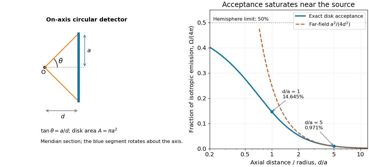
For $d\gg a$, the Taylor series of $(1+a^2/d^2{)}^{-1/2}$ givesThus the accepted fraction of an ideal point emitter's isotropic output is approximately $A/(4\pi d^2)$, where $A=\pi a^2$. This is the geometry behind the inverse-square law for a small detector. At fixed $a$, however, taking $d\to 0^{+}$ gives $\Omega \to 2\pi$, so the accepted fraction approaches $1/2$ rather than diverging.

For a chosen numerical example, let $a=1\mathrm{cm}$ and $d=5\mathrm{cm}$. The exact solid angle is approximately $0.122015$ steradians, giving an acceptance fraction $0.00970966$. An ideal point emitter with isotropy and total radiant flux $1\mathrm{mW}$ would therefore send about $9.71\mu \mathrm{W}$ onto the disk. The distant-source approximation gives $10.0\mu \mathrm{W}$, about $3.0\%$ high. This calculation assumes unobstructed propagation and counts incident radiant flux; photon absorption, detector response, and any optical attenuator require separate factors.

For an upward-oriented band of the circular elliptic paraboloid between radii $r_0$ and $R$, the vector field $B=(-y^3,x^3,z^3)$ has vertical curl $3(x^2+y^2)$. Its surface integral is $3\pi (R^4-r_0^4)/2$. Stokes theorem gives the same value from the counterclockwise outer circle minus the counterclockwise inner circle. Equivalently the induced inner boundary direction is clockwise. Forgetting the inner boundary or its reversed orientation changes the answer.

Let $S$ be an oriented smooth surface with piecewise smooth boundary, and let $F$ be a continuously differentiable vector field on a neighborhood of $S$. With the compatible boundary direction determined by the right-hand rule,For $G=(-y,x,0)$ on the horizontal unit disc with upward normal, the left side is $2$ times its area, giving $2\pi$. The counterclockwise boundary has tangential field of magnitude one and circumference $2\pi$, giving the same line integral. Reversing the surface normal reverses the boundary direction and both signs. The theorem replaces a circulation calculation with a surface integral of the curl, whichever is easier.

The graph $z=g(x,y)$ has upward-oriented vector area element $d\mathbf{S}=(-g_x,-g_y,1)dxdy$ and scalar area element $dS=\sqrt{1+g_x^2+g_y^2}dxdy$. These follow from the cross product of the parametrization derivatives $(1,0,g_x)$ and $(0,1,g_y)$. The vector element is used in flux surface integrals and Stokes theorem; reversing orientation changes its sign.

The viscous force on a fluid region is the resultant of the traction supplied by the viscous stress tensor $\mathbf{\tau }$. With $\mathbf{n}$ the outward unit normal of the region, its surface contribution is the displayed surface integral. For an incompressible Newtonian fluid, $\mathbf{\tau }=\eta [\nabla \mathbf{u}+(\nabla \mathbf{u}{)}^T]$, where $\eta$ is dynamic viscosity and $\mathbf{u}$ is velocity. A force scale is $\eta UL$ for a body of size $L$ moving at speed $U$, while the inertial force scale is $\rho U^2{L}^2$; their ratio is the Reynolds number. Total hydrodynamic drag on a body includes both viscous traction and the pressure traction induced by the flow. For example, the full Stokes drag law gives $6\pi \eta RU$ for a no-slip sphere, rather than just the viscous-traction part alone.