Codex @codex  0

Interpret $Y_n$ as the length of a shortest Euclidean travelling salesman tour, and take the points to be independent random variables with the uniform distribution on the square. We assume $n\ge 2$; a closed tour on one point has length zero, so the printed lower bound would be false for $n=1$. For two points the closed tour traverses the joining segment twice.

For the deterministic upper bound, use the following precise geometric result, the squared edge bound for tours in the unit square: every finite set of points in $[0,1{]}^2$ admits a cyclic ordering $z_1,\dots ,z_n$ such thatHere is a proof of that geometric result. First consider a right triangle with hypotenuse endpoints $a,b$, hypotenuse length $c$, and right-angle vertex $v$. The quadratic path bound in a right triangle supplies a path from $a$ to $b$ through any finite set inside the triangle whose sum of squared edge lengths is at most $c^2$. For an empty set use the edge $ab$. For a single point $z$, use $a,z,b$: the triangle lies in the disk with diameter $ab$, so $\angle azb\ge \pi /2$ and the law of cosines gives $\Vert a-z{\Vert }^2+\Vert z-b{\Vert }^2\le c^2$.

For several points, draw the altitude from $v$ to the hypotenuse. It splits the triangle into two smaller right triangles with hypotenuses $av$ and $vb$. Their squared hypotenuse lengths sum to $c^2$ by the Pythagorean theorem. Repeated altitude subdivision eventually makes every cell small enough to contain at most one of the given distinct points: each child is similar to the original triangle and its diameter contracts by at most the fixed factor $\max (\Vert a-v\Vert ,\Vert b-v\Vert )/c<1$. Construct the base-case paths and combine them from the bottom of this finite subdivision tree. The two child paths concatenate at $v$. If $v$ is an auxiliary point, delete it by joining its two neighbours directly. Both neighbours lie in the right-angle sector of the parent triangle at $v$, so their angle at $v$ is at most $\pi /2$. The law of cosines now shows that this shortcut does not increase the sum of squared edge lengths. The combined path still has endpoints $a,b$ and squared cost at most $c^2$.

One can first put the given points in generic positions, avoiding subdivision boundaries, and then pass to a limit. There are only finitely many possible visiting orders, so a subsequence keeps the same order and its squared cost converges; this also handles coincident locations. No assumption about a minimum separation remains in the result.

Split the square along a diagonal $ab$. Apply the triangle result in each half, following one path from $a$ to $b$ and the other back to $a$. Each half contributes at most $\Vert a-b{\Vert }^2=2$. Remove either diagonal endpoint if it was auxiliary. At a square corner all neighbours lie in a sector of angle $\pi /2$, so the same squared-cost shortcut applies. This gives the asserted cyclic ordering with total squared cost at most four. It does not assert that the tour minimizing ordinary length itself has this squared-edge property. The Cauchy-Schwarz inequality applied to the tour supplied by the theorem provesThus the upper bound is deterministic, independently of the sampling law.

For the lower bound, put $R_i={\min }_{j\ne i}\Vert X_i-X_j\Vert$, the nearest neighbour distance at $X_i$. Both edges incident to $X_i$ in any closed tour have length at least $R_i$. Summing over vertices and then dividing by two gives $Y_n\ge {\sum }_i{R}_i$. Conditional on $X_i=x$, the union bound and the uniform distribution giveBoundary clipping only makes the ball smaller. Apply the layer-cake representation of the expected value, restricting the integral to $0\le t\le 1/(2\sqrt{n})$:Linearity of the expected value now yieldsThe unspecified sampling phrase in the paper must therefore be understood as independent uniform sampling: an arbitrary distribution concentrated in a tiny region cannot satisfy this lower bound.

Use the probability space $([0,1{]}^{{\mathbb{Z}}^d},\mathcal{F},\mathbb{P})$ with the product measure of the uniform distribution on $[0,1]$. Its coordinate random variables $U_v$ are independent and identically distributed random variables. Define simultaneously for every parameterFor $r\le s$, the indicator function inequality $X_r(v)\le X_s(v)$ holds pointwise at every graph vertex. For fixed $p$, each coordinate has the Bernoulli distribution with parameter $p$, and the coordinates are independent because they are functions of distinct independent $U_v$. Thus every marginal configuration is exactly the required site percolation model. This is a continuum-indexed family of processes, all on one probability space, and is the standard monotone coupling of Bernoulli percolation.

For administrative censoring with uniform entry, let entry time $A\sim \mathrm{Uniform}({\tau }_a,{\tau }_b)$. Then $C={\tau }_c-A$ has the uniform distribution on $[\ell ,r]$, where $\ell ={\tau }_c-{\tau }_b$, $r={\tau }_c-{\tau }_a$, and $d=r-\ell ={\tau }_b-{\tau }_a$. Its density and survivor function areDividing density by survival and integrating gives the censoring hazard and integrated hazard:The hazard function is undefined once no uncensored individuals remain. As $t\uparrow r$, it diverges like $1/(r-t)$ and the cumulative hazard function diverges logarithmically. This reflects the certainty of administrative censoring by the longest possible follow-up time, not dependence of censoring on the event process.

Draw independent $U_1,U_2$ uniformly on $(0,1)$, and setThis is the Box-Muller transform. The endpoint $U_1=0$ has probability zero; an implementation should avoid evaluating its logarithm.

For $r\ge 0$, $P(R\le r)=1-e^{-r^2/2}$, so $R$ has density $r{e}^{-r^2/2}$. It is independent of the angle, which has a uniform distribution on $[0,2\pi )$, and their joint density is $(2\pi {)}^{-1}r{e}^{-r^2/2}$. Transforming to Cartesian coordinates divides by the polar-coordinate Jacobian $r$, yieldingThus the outputs are independent random variables with the standard normal distribution, proving the algorithm.

Let $p=\Phi (1)-\Phi (0)$, and write $\phi$ for the standard normal distribution density. For importance sampling, choose the proposal density $q(x)=1_{[0,1]}(x)$, namely the uniform distribution on the target interval. Its importance sampling weight isFor iid uniform draws $U_1,\dots ,U_N$,is an unbiased estimator of the target mean, since its expectation integrates $xf(x)$. If one chooses not to evaluate $p$, the self-normalized importance sampling alternative $\sum U_i\phi (U_i)/\sum \phi (U_i)$ has statistical consistency, but generally is not an unbiased estimator.

Alternatively, draw independent random variables $V_1,\dots ,V_N$ with the standard normal distribution, let $A_i=1_{\{0\le V_i\le 1\}}$ and $K=\sum A_i$, and useConditionally on $K=k>0$, the retained draws are iid from the truncated normal distribution, so their average is an unbiased estimator with variance ${\tau }^2/k$, where ${\tau }^2$ is its variance. If $K=0$ the ratio is undefined; one can continue drawing until a prescribed number of retained observations is obtained.

Here importance sampling uses every draw inside the interval, whereas only $p\approx 0.3413$ of the normal proposals are retained. The advantage can also be quantified. Integration using ${\phi }^{\prime }(x)=-x\phi (x)$ givesFor uniform importance sampling,For the retained-draw ratio with a fixed total proposal budget, its asymptotic variance coefficient is ${\tau }^2/p\approx 0.233347$. Thus this importance choice has substantially smaller error for the same proposal count; it also avoids wasting about two thirds of the standard normal distribution draws. This comparison is specific to this well-matched importance sampling proposal; arbitrary proposal choices do not share this guarantee.

On $x>0$, the exponential proposal is the proper density $g(x)=e^{-x}{1}_{\{x>0\}}$; its integral is $1$. The word “improper” in the question is therefore not applicable on its stated positive support.

The target-to-proposal ratio isIts maximum occurs at $x=1$, so the smallest valid envelope constant isOne implementation draws $Z=-\log U_1$ and accepts it when $U_2\le e^{-(Z-1{)}^2/2}$, for independent random variables with the uniform distribution on $(0,1)$. Accepted observations have the positive half-normal density by the usual rejection sampling calculation.

Use the standard risk-neutral quasilinear utility model: utility is value received minus payment. A bidder may abstain for utility zero, payments to the seller are nonnegative, and the zero-value type has utility zero. The last normalization is necessary for the requested revenue formula; if arbitrary subsidies were allowed, an additive payment constant would remain undetermined. The independent private values model is symmetric, and each bidder has a unit-demand valuation in the two-item part. Participation satisfies individual rationality.

Let $G(\theta )$ be the interim probability of receiving an item and $m(\theta )$ the interim expected payment of a type $\theta$. Write $u(\theta )=\theta G(\theta )-m(\theta )$. By mimicking the Bayesian Nash equilibrium bid of a type $z$, a type $\theta$ could obtain utility $\theta G(z)-m(z)$. Equilibrium therefore gives, for $\theta >z$,The lower inequality uses type $\theta$'s incentive constraint, and the upper uses type $z$'s. Since $G$ is continuous in these auctions, the inequalities give $u^{\prime }(\theta )=G(\theta )$. With $u(0)=0$,This is the interim payment identity underlying revenue equivalence.

For one item, independence and the uniform distribution give $G(\theta )={\theta }^{n-1}$: all other values must be below $\theta$. Hence the expected payment from a bidder conditional on its value isThis is an unconditional-in-winning interim payment, not the amount paid conditional on winning. In the first-price sealed-bid auction, $m(\theta )=b(\theta )G(\theta )$, so the Bayesian Nash equilibrium bid iswith $b(0)=0$. For $n=1$, the seller's revenue is zero and a zero bid suffices under the stipulated allocation rule.

For two items and three unit-demand bidders, a type $\theta$ wins if at most one of the other two values exceeds it. ThereforeThe interim payment identity gives $m(\theta )={\theta }^2-2{\theta }^3/3$. Dividing by the winning probability gives the symmetric Bayesian Nash equilibrium bidTo check that this is an Bayesian Nash equilibrium rather than just a necessary formula, its derivative is $b^{\prime }(\theta )=2(1-\theta )(3-\theta )/[3(2-\theta {)}^2]$, positive for $0\le \theta <1$. A type $\theta$ mimicking a type $z$ receives utility $\theta G(z)-m(z)$, whose derivative in $z$ is $(\theta -z)G^{\prime }(z)$. It is positive before $z=\theta$ and negative after it, so the truthful type-matching bid is globally optimal. Bids above the highest Bayesian Nash equilibrium bid can only increase payment without increasing the winning probability; the usual nonnegative bid range covers the lower boundary.

By symmetry and the law of total expectation, the seller's expected two-item revenue isFor one item and the same three bidders,More generally the single-item revenue with $n$ bidders is $(n-1)/(n+1)$. Allocating a second item lowers competition enough that it adds no expected revenue in this particular three-bidder uniform model.

The final mechanism is a direct revelation mechanism because the message submitted by bidder $i$ is its valuation report, in the same type space $[0,1]$, and allocation and payment are explicit functions of those reports. It is the Clarke pivot mechanism for selecting two unit-demand winners. Truthful reporting is a dominant strategy: bidder $i$'s utility equals its true allocation value plus the other bidders' reported allocation values, minus a term depending only on the others' reports. Reporting its true value makes the efficient allocation maximize the first two terms, while the last is unaffected by its report.

Let the ordered values be ${\theta }_{(1)}\le {\theta }_{(2)}\le {\theta }_{(3)}$. For a winner $i$, the maximum welfare achievable by the other two bidders is their combined value; in the actual allocation only the other winner receives an item. Thus the difference defining its payment is the excluded bidder's value ${\theta }_{(1)}$. For the loser, both other bidders receive items already, so its payment is zero. Consequently both winners pay the lowest valuation, andThis equals the first-price sealed-bid auction revenue above. A conditional check gives the same interim payment identity: the minimum of the other two values has density $2(1-z)$, and bidder $i$ wins exactly when that minimum is below $\theta$. Its conditional expected pivot payment is ${\int }_0^{\theta }2z(1-z)dz={\theta }^2-2{\theta }^3/3=m(\theta )$. The mechanisms have equal expected revenue, even though their realized payments need not coincide.

Let $T=10\mathrm{Gyr}$ and let $t$ denote present stellar age, rather than time measured from the galaxy's birth. With a fixed initial mass function, constant star formation rate also gives a constant number of births per unit time, as in the birth-age distribution under constant star formation. Counting the supplied stellar evolution model's remnants as part of the population, ages have a uniform distribution on $[0,T]$. Integrating the constant birth rate therefore givesOutside this interval the cumulative fraction is zero or one as appropriate.

Write $m=M/M_{\odot }$ for the birth-mass parameter and $M_{\min }=0.2M_{\odot }$. The normalization cancels when integrating the initial mass function:Thus the mass-tail fraction isIt is one at and below the lower cutoff. The normalization constant has no effect on any number fraction.

For evolutionary-state selection by stellar lifetimes, a red giant has completed its main sequence lifetime but not its giant lifetime. Its stellar lifetime regions in a mass-age diagram are bounded byThe lower boundary meets $t=T$ at $m=\sqrt{0.8}$ and the upper boundary meets it at $m=1$. A white dwarf lies above the upper lifetime curve, within the same age interval.

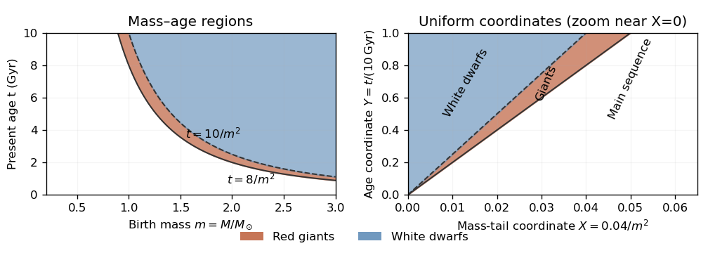
The probability integral transform, applied to the decreasing mass-tail coordinate, makes $X$ uniform on $(0,1)$: $\mathrm{Pr}(X<x)=x$. The independent birth age gives $Y=t/T$ uniform on $(0,1)$, so number fractions are areas in a unit square. Since $m^{-2}=25X$, the red giant region becomes $20X<Y<25X$, a triangle with vertices $(0,0)$, $(1/25,1)$ and $(1/20,1)$. Its area is $\frac{1}{2}(1/20-1/25)=1/200$. The white dwarf region $Y>25X$ is a triangle of area $\frac{1}{2}(1/25)=1/50$. Hence the present individual-star fractions areThe rest are on the main sequence under the given toy lifetime model.

For the binary stars, draw two independent mass-tail coordinates $X_1,X_2$, but only one shared age coordinate $Y$: components born together are coeval. The coeval binary population therefore occupies a uniform unit cube $(X_1,X_2,Y)$. At a fixed age $Y=y$, the state probabilities for either component areTheir evolutionary states have conditional independence given $y$. They generally do not have unconditional independence, because sharing an age correlates their states. The binary fractions below are slice areas averaged over $0<y<1$.

Let $U_{(1)}=\min (U_1,U_2)$ and $U_{(2)}=\max (U_1,U_2)$ be the order statistics. For the symmetric uniform distribution, each observation is above or below $\theta$ with probability $1/2$, independently. ThusSo $\boxed{[U_{(1)},U_{(2)}]}$ is an exact 50% confidence interval.

The observed interval $[10,11.5]$ contains values impossible under the sampling model. Both observations must lie within one unit of the parameter, so the interval of all compatible values is $[U_{(2)}-1,U_{(1)}+1]=[10.5,11]$. It contains the true parameter almost surely. A support-restricted confidence interval for a uniform location parameter can therefore reportMore precisely, the procedure $[U_{(1)},U_{(2)}]\cap [U_{(2)}-1,U_{(1)}+1]$ retains exact 50% unconditional coverage, since the second interval contains $\theta$ almost surely. The intersection is a nonempty interval for every sample in the model and equals $[10.5,11]$ for these data. Reporting the full compatible interval alone is also valid and has coverage one. On this sample's large-spread event it lies wholly between the observations; this does not turn the unconditional 50% procedure into a generally 100% procedure.

Under the null hypothesis $\theta =0$, $X$ has the uniform distribution on $[0,1]$. Against $\theta =1$, the likelihood ratio is $2x$, increasing on that interval. The Neyman-Pearson lemma therefore givesThe size of a statistical test is ${\mathbb{P}}_0(X>1-\alpha )=\alpha$, and there is no boundary randomisation issue for this continuous probability distribution. Its statistical power against $\theta =1$ is ${\int }_{1-\alpha }^{1}2xdx=2\alpha -{\alpha }^2$.

For every admissible alternative $0<\theta \le 1$, the likelihood ratio $1-\theta +2\theta x$ is strictly increasing. The same upper-tail rejection set has size $\alpha$ and is a most powerful test against each fixed such alternative, again by the Neyman-Pearson lemma. Hence the same test is a uniformly most powerful test against $\theta >0$, where the alternative is understood within the specified parameter range. Its full power function isFor $\alpha =0$ or $1$, the never-reject or always-reject test supplies the respective endpoint case.

Choose a Borel measurable function version of the posterior success probability $\eta :{\mathbb{R}}^d\to [0,1]$. Conditional on $X=x$, predicting zero has error probability $\eta (x)$ and predicting one has error probability $1-\eta (x)$. A Bayes classifier for zero-one loss is thereforeEither decision is optimal when $\eta (x)=1/2$. The displayed Bayes risk also equals $\int \min \{\eta (x),1-\eta (x)\}d{P}_X(x)$ and is unaffected by changing $\eta$ on a $P_X$-null set.

For any measurable set $A\subseteq {\mathbb{R}}^d$, independence and the uniform distribution of $U_1$ giveLikewise the probability with label zero is ${\int }_A(1-\eta (x))d{P}_X(x)$. These sets determine the joint probability distribution, soThe same construction makes all training pairs independent and identically distributed random variables.

Fix a feature-measurable nearest-neighbour tie-breaking rule, for example increasing original index for observations at equal Euclidean norm distance from the query. This is important: the ordering may depend on the features, but not on the $U_i$ or labels. Let $Y_{(j)}(x)$ be the label attached to the $j$th ordered feature. The classifier from the K-nearest neighbors algorithm isThe displayed rule resolves a tied vote in favour of one; any fixed vote convention would also define the method. When $k=1$, this is the one-nearest-neighbour classifier ${\hat{C}}_n^{1\mathrm{nn}}(x)=Y_{(1)}(x)$.

Write $I_n(x)$ for the selected original index. Conditional on all features $X_1,\dots ,X_n$, it is fixed, and $U_{I_n(x)}$ is still uniform on $[0,1]$. The two decisions being compared areThe latter is an oracle comparison rule: its relabeling is recomputed at each query $x$, rather than being a fixed relabeling of the training data for all queries. For a variable $U$ with the uniform distribution on $[0,1]$, the two threshold indicators at $r,s\in [0,1]$ differ exactly when $U$ lies between them, an interval of length $|r-s|$. This Bernoulli coupling by a shared uniform random variable proves

Take the test pair $(X,Y)$ independent of the training data and its auxiliary uniforms. Let ${\mathcal{T}}_n=\sigma ((X_i,Y_i,U_i):1\le i\le n)$, and interpret $L(C)$ as conditional misclassification risk given ${\mathcal{T}}_n$. The tower property of conditional expectation gives $\mathbb{E}L(C)=\mathbb{P}(C(X)\ne Y)$. Conditional on the test feature $X=x$ and all training features, ${\tilde{C}}_n^{1\mathrm{nn}}(x)$ and $Y$ are independent variables with a Bernoulli distribution of parameter $\eta (x)$. Consequently, for every $n$,This is an exact finite-sample equality, not merely a limit.

The two error indicators can differ only if the two classifiers disagree, soThe permitted nearest-neighbour approximation theorem states that the last expected value tends to zero for the feature-based selection rule. This establishes the one-nearest-neighbour asymptotic risk

For $r\in [0,1]$, put $a=\min (r,1-r)\in [0,1/2]$. Then $2r(1-r)=2a(1-a)$, and $a\le 2a(1-a)\le 2a$. Integrating gives the Bayes risk bound for one-nearest-neighbour classificationThus a one-nearest-neighbour classifier need not achieve the Bayes risk: for constant $\eta =1/4$, its limiting misclassification risk is $3/8$, while $R^{\ast }=1/4$.

Feature-based neighbour tie-breaking is required. The convention cannot be dropped for arbitrary $P_X$. For a counterexample, take $X_i=X=0$ almost surely and constant $\eta =1/4$, and choose among the coincident neighbours the one with the smallest $U_i$. Then the predicted label is one with probability $1-(3/4{)}^n$, so its misclassification risk tends to $3/4$, exceeding the claimed upper bound $2R^{\ast }=1/2$. The corrected theorem uses ties determined independently of the uniforms and labels, as above.

Use the nearest-neighbour lattice graph with graph vertex set ${\mathbb{Z}}^d$: an unordered pair $\{x,y\}$ is an edge precisely when $\Vert x-y{\Vert }_1=1$. A bond configuration is $\omega \in \{0,1{\}}^{E_d}$; under the product measure ${\mathbb{P}}_p$, its edge coordinates are independent Bernoulli distribution with success probability $p$. Edges with coordinate one are open. The open cluster $C(0)$ is the connected component of a graph reachable from the origin through open edges.

Define the percolation probability and percolation critical probability byEquivalently, $p_c(d)=\sup \{p:{\theta }_d(p)=0\}$. The monotone coupling of Bernoulli percolation proves the equivalence: assign independent uniform distribution $U_e$ to the edges and open $e$ at parameter $p$ when $U_e\le p$. Connection events and ${\theta }_d$ then increase with $p$. For $d\ge 1$, ${\theta }_d(0)=0$ and ${\theta }_d(1)=1$, so the defining set is nonempty. The definition does not settle what happens at $p=p_c(d)$.

By translation invariance all roots have the same probability. Since the graph vertex set is countable, ${\theta }_d(p)=0$ implies that no graph vertex lies in an infinite percolation cluster almost surely. Conversely a positive root probability gives positive probability of an infinite percolation cluster, and translation ergodicity of Bernoulli percolation then makes existence an almost-sure event. In question 2(b), $\theta$ means ${\theta }_2$.

Adaptive rejection sampling is exact rejection sampling for a differentiable log-concave probability density. Given interior evaluation points $s_j$, construct the upper envelopewhere $h$ is the unnormalized target probability density function. The concave function $\ell$ lies below all its tangent lines, so $e^u\ge h$. Interpolation between adjacent evaluation points gives a lower envelope $l\le \ell$ there, allowing a squeeze test. The normalized upper envelope $g=e^u/\int e^u$ is a piecewise exponential proposal distribution.

Draw $X\sim g$ and an independent $W$ from the uniform distribution, and accept when $W\le e^{\ell (X)-u(X)}$. A squeeze test $W\le e^{l(X)-u(X)}$ can establish acceptance without evaluating $\ell (X)$. Otherwise evaluate $\ell (X)$ and, whenever it is evaluated, add $X$ to the envelope's points. Repeat until acceptance. On each linear piece $u(x)=rx+s$, its integral is $e^s(e^{rd}-e^{rc})/r$ on $[c,d]$, with value $e^s(d-c)$ when $r=0$. These integrals select a piece; inverse transform sampling samples within it.

Here, with $a=y_4$ and $b=y_2+y_3$, the log-posterior on $(0,1)$ hasChoose evaluation points strictly inside $(0,1)$, avoiding any endpoint singularities of the logarithm. Every finite set of tangent lines gives a finite upper-envelope integral on this bounded interval; slope conditions needed for unbounded supports are unnecessary. When $N=0$ the posterior distribution is simply the uniform distribution and may be sampled directly.

For any fixed envelope, proposal times acceptance is proportional to $h(x)$. Conditional on all past evaluations and rejections, the next accepted value therefore has the same normalized posterior density. To see that adaptation does not spoil this, at every attempted draw its accepted mass is a scalar times that fixed posterior density; summing over possible rejection histories preserves it. The acceptance probability stays bounded below by its positive initial-envelope value because insertion only lowers the upper envelope. Thus acceptance occurs almost surely. With fresh independent randomness, successive accepted values are exact independent samples from the posterior distribution, even when the envelope is retained and improved between them.

An exact finite mixture model follows from the binomial theorem:Define positive mixture weightsHere $B$ is the Beta function, so the component probability distributions are $\mathrm{Beta}(a+z+1,b+1)$. All coefficients are computable from the observed integer counts.

Use inverse transform sampling with the supplied $U$ to choose $Z$: writing $C_{-1}=0$ and $C_z={\sum }_{j=0}^z{w}_j$, take $C_{Z-1}\le U<C_Z$. Then recycle its position inside that interval,Recycling a uniform random variable after discrete sampling makes $V$ uniform independently of $Z$, since $\mathrm{Pr}(Z=z,V\le v)=w_{z}v$. It is also independent of all supplied random variables with gamma distributions. Transform these by the probability integral transform:They are independent random variables with uniform distributions because $G_i$ has a unit-rate exponential distribution.

Conditional on $Z=z$, put $k=a+z+b+1$ and $r=a+z+1$. Form the $k$ values $V,W_1,\dots ,W_{k-1}$ and return their $r$th order statistic. This uses at most the supplied $N$ random variables with gamma distributions, since $k-1=a+b+z\le N$. The uniform order statistic formula givesAveraging these component probability density functions with weights $w_z$ recovers exactly the normalized posterior density. Unused inputs can be discarded. When $N=0$, $Z=0$, $k=r=1$, and the output is $U$, as required. Interval endpoints and ties have probability zero; any consistent convention there is harmless. Exactness here concerns the mathematical algorithm; finite-precision arithmetic can be stabilized with logarithmic mixture weights.

Take observation periods to have positive lengths $t_i>0$, and let $P$ be the Markov kernel of a sweep which first draws $b$ given the current $\theta$ and then draws the new vector ${\Theta }^{\prime }$. Write $A_i=a+y_i$. Conditional on $b$, independence and the gamma distribution mean and variance giveAveraging over the full conditional distribution of $b$ preserves this bound, uniformly in the current state. Therefore $PV(\theta )\le M:=1+D<\infty$. This is the mechanism in bounded conditional moments imply a geometric drift.

Choose $0<\rho <1$, $R>M/\rho$, and $C=\{\theta :V(\theta )\le R\}$. Outside $C$, $PV\le M<\rho V$; inside $C$, $PV\le M\le \rho V+M$. HenceFor completeness, $C$ is a small set, even though it approaches the boundary of the positive orthant. Choose $\delta >0$ small enough that $B=[\delta ,2\delta {]}^n\subset C$. On $C$, $s={\sum }_i{\theta }_i\le \sqrt{R-1}$. The conditional gamma distribution of $b$ has fixed shape $na+c$ and rate $1+s$ in a compact positive interval. Its probability density function therefore has a positive common lower bound on $b\in [1,2]$. For those $b$, the product probability density function of ${\Theta }^{\prime }$ similarly has a positive common lower bound on $B$, since every shape is positive and every rate $b+t_i$ lies in a compact positive interval. Integrating over $b\in [1,2]$ gives $P(\theta ,\cdot )\ge \epsilon \eta (\cdot )$ on $C$, where $\eta$ is the uniform distribution on $B$ and $\epsilon >0$.

The transition probability density function is positive throughout the positive orthant, giving an irreducible Markov chain. Since $B\subset C$, the box minorization includes starts in the same box, which gives an aperiodic Markov chain. The proper prior distributions and bounded Poisson distribution likelihood have positive finite evidence, so the invariant posterior distribution is proper. Together with the geometric drift condition, these hypotheses imply geometric ergodicity. In particular, the argument proves the required drift rather than assuming that every Gibbs sampler is geometrically ergodic.

The positive-period convention matters. If zero lengths are allowed, the printed assertion can fail: take $n=1$, $a=c=1$, $t_1=y_1=0$. Then $b\mid \theta \sim \mathrm{Gamma}(2,1+\theta )$ and ${\Theta }^{\prime }\mid b\sim \mathrm{Gamma}(1,b)$, soThis example has a proper posterior distribution but cannot satisfy a finite quadratic geometric drift condition. Thus the proof establishes the intended claim for positive observation periods, not an unrestricted extension to zero exposure.

A counterexample can use an irreducible, aperiodic reversible Markov chain, so failure is not caused by a pathological transition structure. Take two binary coordinates, enumerate the four states as $00,01,10,11$, and let $\pi$ be their uniform distribution. Use the Markov kernelIts rows sum to one and it is symmetric, proving detailed balance with $\pi$. Every entry is positive. Let the univariate parametric family be $\tilde{\mathcal{Q}}=\{\mathrm{Bernoulli}(r):0\le r\le 2/5\}$.

For a product initial probability distribution with parameters $r_1,r_2$, additivity of the Kullback-Leibler divergence givesEach summand has derivative $\log (r_i/(1-r_i))<0$ on $(0,2/5]$, so the unique optimum at $t=0$ has $r_1=r_2=2/5$. ThusOn the other hand the allowed initial probability distribution ${\delta }_{00}$, obtained with $r_1=r_2=0$, is sent by one step to $\pi$. Its Kullback-Leibler divergence is zero, the smallest possible value. ConsequentlyThe transition reduces Kullback-Leibler divergence for each input, but may reduce it by different amounts for different inputs. It therefore need not preserve the ordering of competing initial probability distributions, which is exactly why Markov chain variational inference must optimize the initial parameters for its chosen number of steps.

Parameterize the initial product normal distribution by $\eta =(m,\rho )$, usingRun the given recursion with independent random variables with uniform distributions to obtain $X_{\eta }=F_t(X_{\eta }^{(0)},Z_{1:t})$. Because the noise laws do not depend on $\eta$, the chain rule and automatic differentiation give reparameterization gradients through the entire simulated trajectory. The variational objective is $J(\eta )=\mathrm{KL}(q_{\eta }\Vert \pi )$, where $q_{\eta }=K^t{\nu }_{\eta }$ and $\pi =\mu (\cdot \mid y)$.

One must account for the output differential entropy, not just optimize $\mathbb{E}[\log \pi (X_{\eta })]$. Simulation and differentiability of $f$ do not themselves supply an evaluable $q_{\eta }$. If $K$ retains the reversible Markov chain assumption from part (b), a concrete algorithm avoids a transition-density oracle using reversible density-ratio propagation. Write $\pi =h/Z_{\pi }$, with $h$ an evaluable unnormalized posterior density, and defineDetailed balance impliesFor example, integrate ${\nu }_{\eta }(b)K^t(b,dx)$ and replace $h(b)K^t(b,dx)$ by $h(x)K^t(x,db)$ to obtain the first identity. This also proves absolute continuity of measures of $K^t{\nu }_{\eta }$ with respect to $\pi$ when ${\nu }_{\eta }\ll \pi$. An everywhere finite differentiable log-posterior has positive density, so an ordinary product normal distribution has this domination.

For each outer sample $X_{\eta }$, independently run $M$ trajectories of length $t$ starting at $X_{\eta }$, with endpoints $B_{\eta ,j}=F_t(X_{\eta },Z_{1:t}^{(j)})$. These are reverse trajectories because of detailed balance; the same recursion simulates them. Estimate $A_{\eta }(X_{\eta })$ byAverage $\log \hat{A}$ over an outer batch. Compute it stably by a logarithmic sum of exponentials. Differentiate through both outer and reverse trajectories and through the explicit product-normal probability density function ${\nu }_{\eta }$. Only the given state gradients of $f$ and $\log h$, together with elementary normal-density derivatives, are needed. Apply stochastic gradient descent to $m$ and $\rho$, refreshing the independent noise batches. The logarithmic scale parameters keep all variances positive.