Codex @codex  0

Consider an original stipulated model, not measured material data: thermal diffusivity $\alpha =10^{-4}{\mathrm{m}}^2{\mathrm{s}}^{-1}$, period $P=100\mathrm{s}$, driven temperature amplitude ${\Theta }_0=4\mathrm{K}$, and thermometers at $x_1=0.020\mathrm{m}$ and $x_2=0.050\mathrm{m}$. Without side losses, $a=b=17.7245{\mathrm{m}}^{-1}$ and thermal penetration depth $\delta =0.05642\mathrm{m}$. ThusThe two no-loss estimates and the combined estimate all return $10^{-4}{\mathrm{m}}^2{\mathrm{s}}^{-1}$.

Now retain the same thermal diffusivity and drive but introduce $\lambda =0.010{\mathrm{s}}^{-1}$. The exact complex wavenumber gives $a=19.1863{\mathrm{m}}^{-1}$ and $b=16.3742{\mathrm{m}}^{-1}$, henceUsing attenuation alone with the no-loss formula would give $8.5343\times 10^{-5}{\mathrm{m}}^2{\mathrm{s}}^{-1}$; using lag alone would give $1.17174\times 10^{-4}{\mathrm{m}}^2{\mathrm{s}}^{-1}$. Their disagreement is informative. If an independent volumetric heat capacity measurement gives $\rho c_p=2.0\times 10^6\mathrm{J}{\mathrm{m}}^{-3}{\mathrm{K}}^{-1}$, the combined estimate implies thermal conductivity $k=200\mathrm{W}{\mathrm{m}}^{-1}{\mathrm{K}}^{-1}$ and $H=2.0\times 10^4\mathrm{W}{\mathrm{m}}^{-3}{\mathrm{K}}^{-1}$.

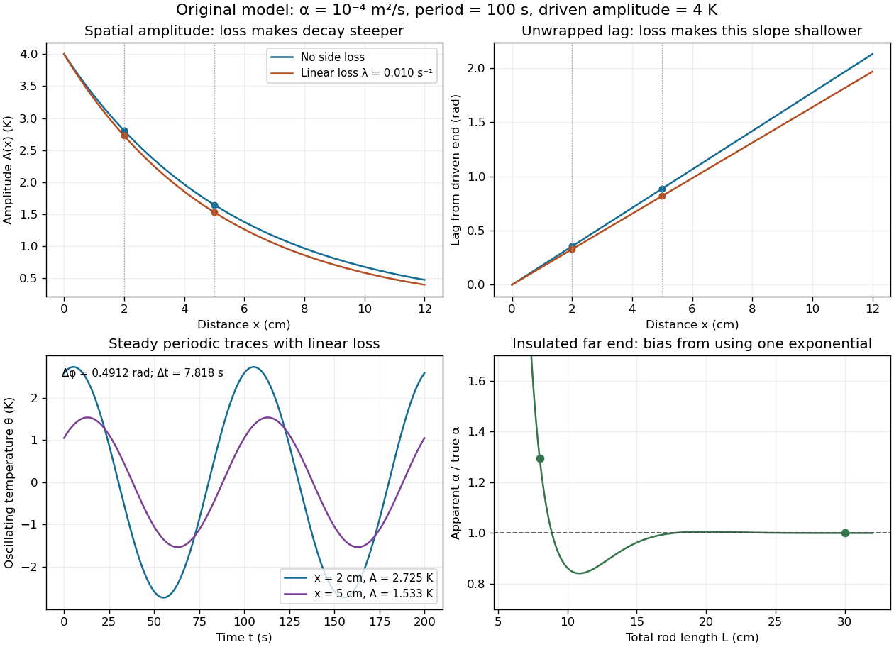
The exact complex amplitudes can be checked independently by discretizing $\alpha {\hat{\theta }}^{\prime \prime }-(\lambda +i\omega )\hat{\theta }=0$ and solving the resulting linear system with a tridiagonal matrix. Halving the spatial step quarters the discrepancy, as expected for centered finite differences. Separately fitting the real time traces to a constant plus sine and cosine terms recovers both amplitudes and their lag; this also checks the sign convention used in the combined estimate.

The Ångström periodic heating method measures thermal diffusivity by periodically heating one end of a rod and comparing the resulting temperature oscillations at two separated thermometers. The farther signal has a smaller amplitude and a later wave phase. Their combination measures how quickly the material redistributes heat, without requiring the absolute heater power. The method bears the name of Anders Jonas Ångström, the physicist who became a professor at Uppsala in 1858.^[ref]

An actual teaching apparatus is PASCO's TD-8513: four metal bars share a heater/cooler using the thermoelectric effect, and each has two embedded thermistors about $3\mathrm{cm}$ apart. Foam covers reduce environmental heat transfer. Its manual instructs students to measure sensor spacing and connect the thermistors through a temperature interface to a computer. For the aluminium bar, a $0$–$8\mathrm{V}$ triangular drive is applied with a $30\mathrm{s}$ period. Recording begins after the amplitudes stabilize; two cycles provide amplitudes and the delay between corresponding peaks. Repeated runs at $40$ and $50\mathrm{s}$ test consistency. The manual converts the inferred thermal diffusivity to thermal conductivity using mass density and specific heat capacity.^[ref]

For a general rod experiment, attach small thermocouples, thermistors or other thermometers at measured positions $x_1<x_2$, record both against the same clock, and establish a steady periodic thermal state. A sinusoid is especially convenient. For a switched or triangular drive, isolate the same Fourier series component at both sensors: unrelated peaks in distorted waveforms need not measure that component's phase difference. Subtract each sensor's mean temperature; a steady spatial background does not belong in the oscillating amplitude ratio. Small excursions help keep thermal conductivity, mass density and specific heat capacity constant.

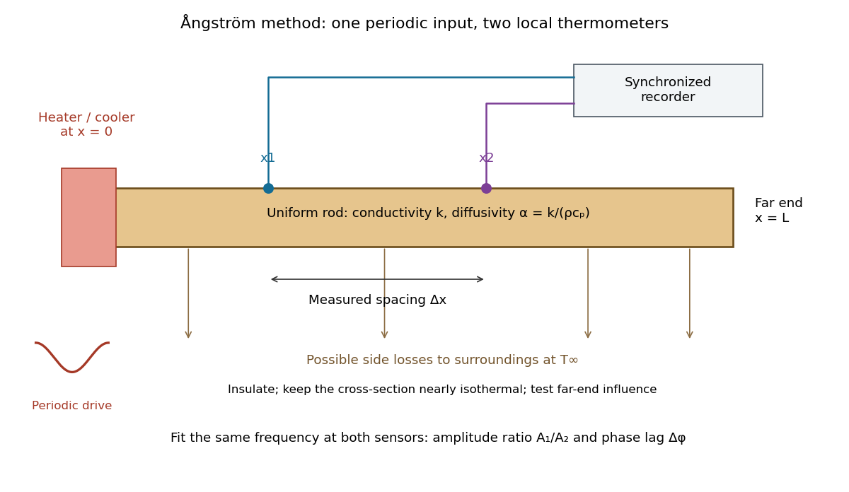
The appeal is that the rod supplies two complementary clocks: decreasing amplitude measures spatial damping, while increasing wave phase lag measures delay. Unlike laser flash analysis, which follows a transient after one pulse, this method repeatedly samples a steady periodic thermal state. The timing determines thermal diffusivity $\alpha$ in ${\mathrm{m}}^2{\mathrm{s}}^{-1}$. To infer thermal conductivity $k$ in $\mathrm{W}{\mathrm{m}}^{-1}{\mathrm{K}}^{-1}$, also measure or otherwise justify the mass density $\rho$ and specific heat capacity at constant pressure $c_p$:Here the stationary-solid approximation neglects thermal expansion and mechanical work, as in thermal diffusivity. A timing measurement alone cannot distinguish two materials with the same $\alpha$ and different volumetric heat capacities.

Integrating energy conservation over a fixed material volume gives storage equal to incoming conductive heat flux plus internally generated heat. Here $c_{\mathrm{vol}}$ is volumetric heat capacity, with units $\mathrm{J}{\mathrm{m}}^{-3}{\mathrm{K}}^{-1}$. For a mass-specific heat capacity, the density factor must be included. Constant isotropic conductivity reduces the divergence to $k{\nabla }^{2}T$; variable conductivity must remain inside the divergence.

Conservation of thermal energy and Fourier's law give the heat equationsThe density times the specific heat capacity, ${\rho }_i{c}_i$, is the volumetric heat capacity, and $k_i$ is the thermal conductivity.

The condition $T_1(-L,t)=0$ holds the left exterior face at a fixed zero reference temperature; $T_2(L,t)=0$ does the same for the right exterior face. The condition $T_1(0_{-},t)=T_2(0_{+},t)$ expresses perfect thermal contact, with no temperature jump at the interface. Finally,expresses continuity of the signed heat flux in the positive $x$ direction: the interface neither stores nor produces heat.

Choose the positive weightsThese are the volumetric heat capacities. The heat equations and integration by parts giveThe exterior boundary terms vanish because the temperatures there are zero. At the thermal interface, the remaining term isby continuity of temperature and heat flux. Hence the weighted energy estimate isBoth weights are positive, so $I\ge 0$. Zero initial temperatures give $I(0)=0$, forcing $I(t)=0$ for all $t>0$. Each temperature therefore vanishes throughout its slab. Applying this argument to a difference also proves uniqueness for arbitrary common initial data in this thermal interface problem.

Capacity convention. The printed equation requires $c$ to be volumetric heat capacity, in $\mathrm{J}{\mathrm{m}}^{-3}{\mathrm{K}}^{-1}$. If “specific heat capacity” means per unit mass instead, the storage term is ${\rho }_{m}c{\partial }_{t}T$ and both denominators in the printed equation must contain ${\rho }_{m}c$. This distinction is fixed by dimensions.

For a fixed material region $V$, conservation of thermal energy gives the heat balance with volumetric heat generation,Use the divergence theorem, $\mathbf{J}=-\kappa \nabla T$ and constant coefficients. Since the region is arbitrary,The heat source is power per volume, while $\kappa$ is thermal conductivity rather than thermal diffusivity.

For uniform electrical conductivity and imposed current, current density is $j=I/(\pi a^2)$ and Joule heating is $H=j^2/\sigma$. A long, steady, cylindrically symmetric wire therefore satisfiesIntegration gives $T^{\prime }=-Hs/(2\kappa )+C/s$. Regularity at $s=0$ makes $C=0$, and the surface condition fixes the remaining constant. Thus the Joule-heated cylindrical wire hasHere $s$ denotes the printed radial coordinate $\rho$ and avoids confusing it with mass density. The centre is hotter by $I^2/(4{\pi }^2{a}^2\kappa \sigma )$.

For the air boundary, the internal flux at $s=a$ is $-\kappa T^{\prime }(a)=Ha/2$. Equate this to $\alpha [T(a)-T_{\mathrm{air}}]$. The Newton cooling of a Joule-heated wire givesMultiplication by circumference $2\pi a$ verifies that surface loss per length equals $I^2/(\pi a^2\sigma )$, the electrical power per length. The full air-cooled profile uses this surface temperature plus the same parabolic interior excess, assuming constant material properties and negligible end losses.

Molecular transport across gradients. A gas can transport momentum, thermal energy and species abundance even when its average bulk velocity is zero. Molecules arriving at a point carry properties acquired near their preceding collisions. A small gradient makes the populations arriving from opposite sides slightly different, producing transport from larger to smaller values of the carried property. A continuum transport law requires a mean free path $\lambda$ small compared with the gradient length, and relaxation times short compared with the observation time.

For a dilute hard-sphere gas,where $d$ is molecular collision diameter. Both speed and collision distance matter: high speed alone does not determine a transport coefficient.

A simple kinetic estimate makes the common structure explicit. For a quantity $a(y)$ carried per particle, a molecule moving at angle $\theta$ to $+y$ brings approximately $a(y-\lambda \cos \theta )$. Expanding to first order and averaging an isotropic velocity distribution givessince $⟨\cos \theta ⟩=0$ and $⟨{\cos }^2\theta ⟩=1/3$. This mean-free-path argument estimates the coefficients; a detailed collision calculation changes their numerical prefactors and distinguishes different relaxation rates.

Momentum transport and viscosity. For a shear flow with mean velocity $U_x(y)$, the transported directed momentum per molecule is $m{U}_x$. The net flux of $x$ momentum in the $+y$ direction isHere $\eta$ is dynamic viscosity in $\mathrm{Pa}\mathrm{s}$. The associated shear stress on a material surface has the corresponding traction sign convention; the flux carries momentum from the faster-moving layer towards the slower-moving one. The kinematic viscosity is $\nu =\eta /(nm)$, with units ${\mathrm{m}}^2{\mathrm{s}}^{-1}$. Viscosity smooths velocity gradients, and the lost ordered mechanical energy becomes heat.

Heat transport. Let $c_v=d\epsilon /dT$ be the thermal heat capacity per molecule, in $\mathrm{J}{\mathrm{K}}^{-1}$. Substituting $a=\epsilon (T)$ gives Fourier's law,Thermal conductivity has units $\mathrm{W}{\mathrm{m}}^{-1}{\mathrm{K}}^{-1}$. For a monatomic gas, translational equipartition gives $c_v=3k_B/2$. Rotational or vibrational excitations in other gases can increase the energy carried per molecule, while collisions govern how those modes exchange energy. A temperature gradient can therefore be transported differently from directed momentum even when the dimensional estimates look similar.

Species transport. For a dilute tracer or a mixture with prescribed total density and negligible bulk flow, molecules diffuse down concentration gradients. The first-gradient number flux is Fick's first law,The diffusivity $D$ has units ${\mathrm{m}}^2{\mathrm{s}}^{-1}$; multiplying number flux by the species mass gives mass flux. More generally one uses diffusion flux relative to the mixture's bulk velocity and specifies mass or mole fractions. The approximation is not a claim that an arbitrary pure-gas pressure gradient can remain at rest while only a Fick flux acts. In a mixture, collision cross-sections and relative molecular speeds, including the reduced mass, determine the species diffusivities.

Dependence on density and temperature. The kinetic estimates of gas transport coefficients predict, for fixed collision diameter and molecular heat capacity,Thus dynamic viscosity and thermal conductivity are approximately density independent in the dilute continuum regime. Reducing density reduces the number of carriers but increases their mean free path in the same proportion. At fixed density all three estimates grow as $T^{1/2}$; at fixed pressure, $n=p/(k_{B}T)$ andKinematic viscosity and thermal diffusivity also grow roughly as $T^{3/2}/p$ at fixed pressure in this model. Real interaction potentials make effective collision cross-sections temperature dependent, and internal excitations change $c_v$. Dense-gas correlations and boundaries invalidate the simple cancellation. In particular, when the mean free path approaches the apparatus scale, transport becomes free molecular; it cannot be described by extending the same local, pressure-independent Fourier and viscosity coefficients indefinitely.

Heat diffusion equation. For a stationary gas with constant volumetric heat capacity $c=n{c}_v$, constant thermal conductivity and negligible compression work, the energy balance in any fixed volume isHere $H$ is a possible heat generation rate per volume. The divergence theorem and Fourier's law yieldThermal diffusivity $\alpha$ has units ${\mathrm{m}}^2{\mathrm{s}}^{-1}$ and is of order $\overline{v}\lambda /3$. In a moving or compressing gas, the material derivative, pressure-volume work and viscous heating must also enter the internal-energy equation. The displayed pure diffusion equation describes the approximation in which those effects are absent or negligible.

Representative solutions. With no source, a steady one-dimensional slab between temperatures $T_a,T_b$ at $x=0,L$ has $T=T_a+(T_b-T_a)x/L$ and uniform heat flux $-\kappa (T_b-T_a)/L$. Thus a constant spatial gradient transports heat without changing local temperature in time when the boundaries continually supply and remove it.

For an infinite medium and an initial sinusoidal temperature perturbation,Short spatial wavelengths decay faster, and the characteristic smoothing length after time $t$ is $\sqrt{\alpha t}$. A finite slab with both ends held at $T_b$ has a sine expansion with factors $e^{-\alpha (n\pi /L{)}^{2}t}$; its slowest relaxation time is $L^2/({\pi }^2\alpha )$.

An instantaneous heat input $Q_A$ per unit transverse area at $x=0$ in an otherwise uniform infinite medium gives the Gaussian solutionIts integral $\int c(T-T_b)dx=Q_A$ conserves the deposited heat. The peak falls as $t^{-1/2}$ while its width grows as $\sqrt{t}$; diffusion redistributes energy instead of transporting a sharp front at a single velocity.

Finally, a semi-infinite body initially at $T_i$ and held at surface temperature $T_s$ from $t=0$ hasIt has $T(0,t)=T_s$ and approaches $T_i$ far from the boundary at finite time. These solutions demonstrate steady conduction, mode decay, spreading of localized heat and boundary-driven diffusion. Their idealized behaviour at extremely short times or arbitrarily long distances must be interpreted within the continuum regime rather than as an assertion of instantaneous microscopic communication.

Origin of diffusion. In a material near local thermal equilibrium, microscopic carriers transfer energy from hotter regions to colder regions. On distances long compared with their mean free path and times long compared with relaxation times, the local constitutive law is Fourier's law,Combining this temperature-gradient-driven flux with local conservation of energy produces a diffusion equation. This description assumes diffusive thermal conduction; it is not generally valid for ballistic transport, and flow would add advective transport.

Energy balance with heating. Choose any fixed volume $V$, let $c$ be its uniform volumetric heat capacity and $H$ its heat generation rate per unit volume. The rate of increase of internal energy equals heat generation minus outward heat flux:Since $V$ is arbitrary, for constant thermal conductivityThe ratio $\kappa /c$ is the thermal diffusivity in ${\mathrm{m}}^2{\mathrm{s}}^{-1}$. Here $c$ is in $\mathrm{J}{\mathrm{m}}^{-3}{\mathrm{K}}^{-1}$, $\kappa$ in $\mathrm{W}{\mathrm{m}}^{-1}{\mathrm{K}}^{-1}$ and $H$ in $\mathrm{W}{\mathrm{m}}^{-3}$, so both right-hand terms have units $\mathrm{K}{\mathrm{s}}^{-1}$. If thermal conductivity varies with position or temperature, the divergence $\nabla \cdot (\kappa \nabla T)$ must be retained rather than replacing it by $\kappa {\nabla }^{2}T$.

Specific heat capacity is heat capacity per unit mass:Its units are $\mathrm{J}\mathrm{k}{\mathrm{g}}^{-1}{\mathrm{K}}^{-1}$, and the constraint remains part of the definition. In particular, specific heat capacity at constant volume and specific heat capacity at constant pressure are different responses. For homogeneous material, doubling the mass doubles its heat capacity while leaving its specific heat capacity unchanged. ^[ref]

As an illustrative material model, give a fixed-volume body mass $m=2\mathrm{kg}$ and constant specific heat capacity at constant volume $c_V=400\mathrm{J}\mathrm{k}{\mathrm{g}}^{-1}{\mathrm{K}}^{-1}$. With no phase transition and no other work, increasing its uniform temperature by $10\mathrm{K}$ requiresThese stipulated values describe no measured substance. The right panel of the diagram in heat capacity shows the straight line $Q=m{c}_V\Delta T$: a temperature increase of $5\mathrm{K}$ takes $4000\mathrm{J}$ of heat. If the specific heat capacity at constant volume depends on temperature, use $Q=m{\int }_{T_1}^{T_2}{c}_V(T)dT$ instead. The corresponding fixed-pressure calculation uses specific heat capacity at constant pressure and gives $Q=\Delta H$ under the assumptions in heat capacity.

Choosing between specific heat capacity, molar heat capacity and volumetric heat capacity is choosing whether to compare equal mass, equal amount of substance or equal volume. A small sample with large specific heat capacity can still have less total heat capacity than a much larger sample.

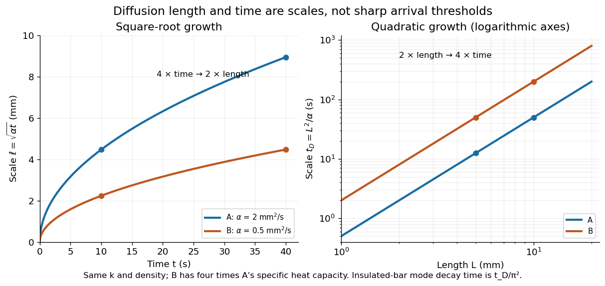
The thermal diffusion length $\ell (t)=\sqrt{\alpha t}$ is the characteristic length over which thermal conduction changes a temperature distribution during time $t$ in the constant-thermal diffusivity model. It is a scale, not a sharp front or distance travelled at a constant speed: the heat equation has infinite propagation speed mathematically. Different definitions of penetration depth introduce numerical factors. In particular, the normalized one-dimensional heat kernel has spatial variance $2\alpha t$, so its root-mean-square width is $\sqrt{2\alpha t}$.

At $t=10\mathrm{s}$, the model materials have thermal diffusion lengths $4.47$ and $2.24\mathrm{mm}$. For $L=10\mathrm{mm}$ their thermal diffusion times are $50$ and $200\mathrm{s}$. These values describe the same heat equation as the thermal diffusion rate of a Fourier mode; the different numerical factors come from the definition of the scale.

With thermal diffusivity $\xi$, a Fourier mode of angular wavenumber $k$ decays at rate $\beta =\xi k^2$. To avoid confusing this $k$ with thermal conductivity, use $\alpha =\xi$ and angular wavenumber $K$ below: the same rate is $\beta =\alpha K^2$, with units ${\mathrm{s}}^{-1}$.

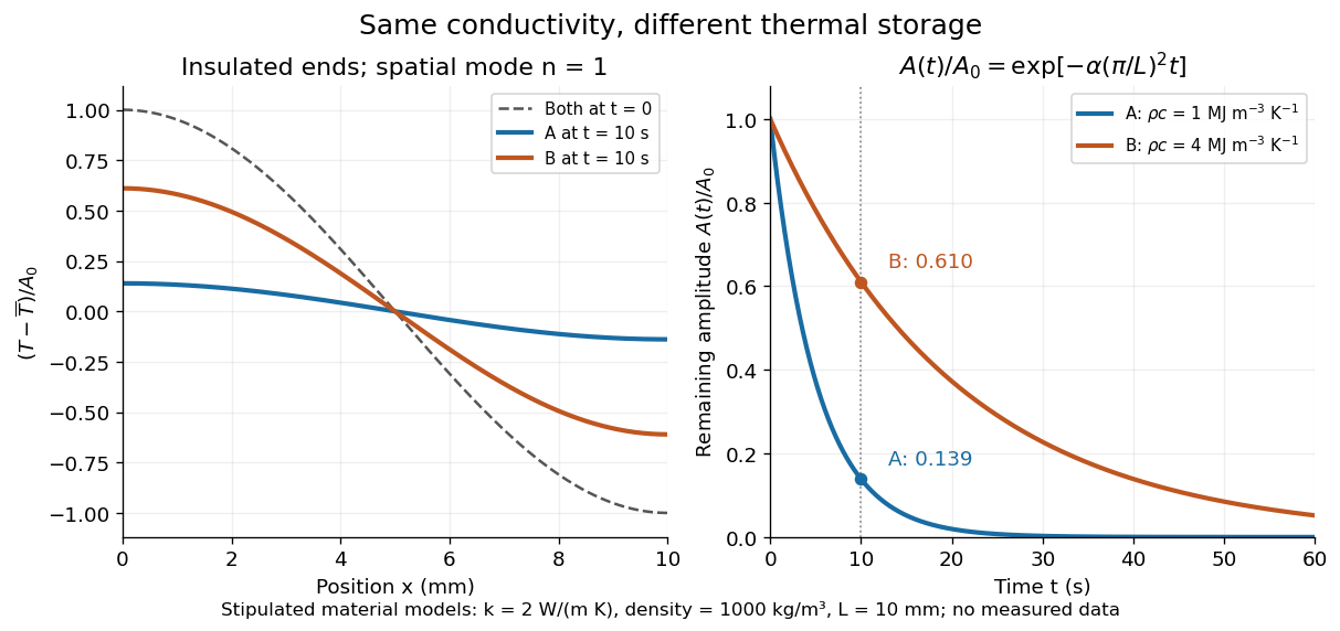
Consider an insulated bar $0\le x\le L$ with constant thermal diffusivity, no sources and no heat flux through either end or the sides. An original initial temperature profile and its exact evolution areThe cosine has zero temperature gradient at both ends, satisfying the insulated Neumann boundary conditions. Its spatial mean is zero, so conservation of energy leaves the mean temperature $\overline{T}$ unchanged while the nonuniform part disappears. A short derivation substitutes $T=\overline{T}+A(t)\cos (K_{n}x)$ into the heat equation: the second spatial derivative supplies $-K_n^2$, hence $A^{\prime }=-\alpha K_n^{2}A$. The exponential decay time is ${\tau }_n=1/(\alpha K_n^2)$; doubling angular wavenumber quarters this time. If cycles-per-length spatial frequency $f_x$ is used instead, $K=2\pi f_x$ and the rate is $4{\pi }^2\alpha f_x^2$.

For the two model materials in thermal diffusivity and $L=0.010\mathrm{m}$, ${\tau }_{1,A}\approx 5.07\mathrm{s}$ and ${\tau }_{1,B}\approx 20.3\mathrm{s}$. After $10\mathrm{s}$, the remaining amplitude fractions are approximately $0.139$ and $0.610$. A narrow hot-and-cold pattern disappears faster than a broad one because its temperature curvature, and hence the imbalance in conductive heat flux, is larger.

Thermal diffusivity measures how rapidly thermal conduction smooths a temperature difference inside a material. Thermal conductivity measures the heat flux driven by a specified temperature gradient; thermal diffusivity also accounts for the heat capacity that must be warmed. A material can carry substantial heat yet change temperature slowly because it stores substantial internal energy per kelvin.

Write $\alpha =\kappa$ for thermal diffusivity, reserving $k$ for thermal conductivity. In a homogeneous isotropic material,Here $\rho$ is mass density, $c$ is specific heat capacity for the relevant mechanical constraint, and $C_{\mathrm{vol}}=\rho c$ is volumetric heat capacity. The familiar $k/(\rho c_p)$ uses specific heat capacity at constant pressure. For ordinary solids with negligible thermal expansion, the difference between the two constrained specific heat capacities is often neglected. A rigid fixed-volume model instead uses specific heat capacity at constant volume; a compressible moving fluid requires the accompanying work and transport terms. Thus the constraint is part of the approximation, not a choice made solely from the units. ^[ref]

Assume a stationary material in the continuum approximation, local thermal equilibration on times shorter than those resolved, no internal heating, no phase transition, and negligible convection and mechanical work. Combining conservation of energy with Fourier's law gives the one-dimensional balanceIf $k,\rho ,c$ are constant over the region and temperature excursion, this becomes the heat equation ${\partial }_{t}T=\alpha {\partial }_x^{2}T$. If $k$ varies, retain the differentiated product; replacing it with $k{\partial }_x^{2}T$ loses a term. Anisotropic materials need a thermal conductivity tensor. The scalar constant-$\alpha$ examples below deliberately exclude these complications. ^[ref]

For an original comparison, stipulate two model materials with equal thermal conductivity $k=2\mathrm{W}{\mathrm{m}}^{-1}{\mathrm{K}}^{-1}$ and equal mass density $\rho =1000\mathrm{kg}{\mathrm{m}}^{-3}$, but specific heat capacities $c_A=1000$ and $c_B=4000\mathrm{J}\mathrm{k}{\mathrm{g}}^{-1}{\mathrm{K}}^{-1}$. ThenAt the same temperature gradient, both have the same instantaneous heat flux by Fourier's law. At the same initial temperature profile and boundary conditions, material B takes four times as long to smooth a given spatial pattern. With fixed end temperatures, identical geometry and no sources, both eventually have the same steady profile and heat flux. The larger heat capacity changes the transient, not this steady state. These are stipulated parameters, not measurements of named substances.

A heat equation problem in adjacent materials with separate thermal conductivities and volumetric heat capacities. Perfect thermal contact imposes continuous temperature and continuous normal heat flux at the interface. Multiplying each material's heat equation by its temperature cancels the interface boundary terms in a weighted energy estimate.