Topics (384k) Articles (398k) Users (410) Discussions (242) Comments (383) Files (13k) New article

Detector volume averaging is the spatial averaging of a nonuniform radiation field over a detector's finite sensitive region. A reading associated with the detector centre need not equal the local absorbed dose at that point. This limits spatial resolution even if the detector position and electronic readout are exact.
For an idealized linear response, let be the absorbed dose field in the undisturbed medium and let be a normalized spatial weighting function, with . Model the spatially averaged quantity byThe model separates averaging from the change in the radiation field caused by inserting the detector. A real ionization chamber can require both effects to be considered. The IAEA definition compares a point dose with the average over the detector's sensitive volume, both evaluated in water with the detector absent.[ref]
Dosimetry of Small Static Fields Used in External Beam Radiotherapy by the International Atomic Energy Agency. §3.1.4, printed p. 37, definition and spatial weighting in equation (5)
For an original one-dimensional example, suppose the detector averages uniformly over a full width . ThenAn ideal sharp edge , where is the Heaviside step function, is recorded asThus a detector gives a distance between the 20-percent and 80-percent response points, although the stipulated field edge has zero transition width. A detector gives in the same model.
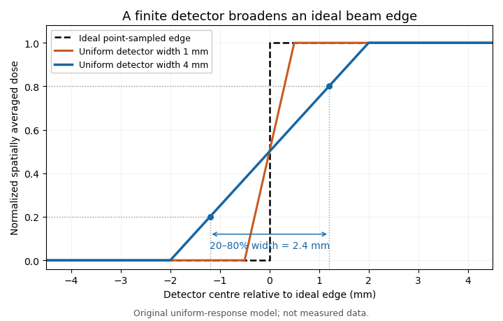
Uniform finite-detector averaging turns a sharp radiation-field edge into a ramp. Original model calculation; the indicated 2.4 mm width belongs to the 4 mm detector, not to an intrinsic field transition.
Details. For a smooth field, a Taylor expansion under the symmetric uniform weighting gives . A constant slope averages to its centre value; curvature produces the leading local discrepancy. A detector-volume-averaging correction factor therefore depends on the field shape and detector geometry, rather than only on the detector's nominal volume.
A proposed apparatus test scans a stable radiation field with detectors of different effective widths or orientations, keeping depth and irradiation geometry fixed. Changes in the recorded edge width test spatial response, while a uniform region checks relative sensitivity. The IAEA's geometric weighting examples show why a projected detector area may need nonuniform weighting; finer scan steps alone cannot remove averaging within each reading.[ref]
A potassium channel is an ion channel that preferentially conducts potassium ions. Its selectivity filter can compensate for the energetic cost of removing water from an ion, while discriminating between ions of different geometry. A crystal structure of a bacterial potassium channel revealed how repeated backbone oxygen atoms line the narrow filter. [ref]
Different potassium channels open under different conditions. Leak channels contribute to resting membrane potential, whereas voltage-dependent channels can support repolarization after an action potential. The direction of current depends on voltage relative to the potassium reversal potential, not simply on the channel's name. Selectivity and gating describe different aspects of its function.
A sodium channel is an ion channel that preferentially conducts sodium ions. In a voltage-gated sodium channel, changes in membrane potential control opening and inactivation. Under usual neuronal conditions, opening permits inward current that promotes depolarization, recruiting more voltage-gated sodium channels during the rising phase of an action potential. [ref]
Molecular Biology of the Cell, 4th edition by Bruce Alberts and others. Chapter 11, Voltage-Gated Ion Channels Generate Action Potentials in Electrically Excitable Cells
An illustrative current relation is , with an explicitly chosen sign convention. Even a large conductance produces little net current near the sodium reversal potential. Channel availability, opening and ionic driving force are therefore distinct. Inactivation also differs from merely closing a resting activation gate: recovery depends on the preceding voltage history.
A channelrhodopsin is a light-gated ion channel associated with a retinal chromophore. Absorbing light changes the protein's conducting state, connecting photoreception directly with ion movement across a cell membrane. Naturally occurring members in Chlamydomonas reinhardtii participate in responses to illumination.[ref]
The landmark channelrhodopsin-2 study expressed the protein in Xenopus laevis oocytes and mammalian cells and recorded light-evoked electric currents. Altering ionic conditions showed passage of multiple cations; continued illumination produced an initial response followed by a smaller sustained conductance. Expressing the channel in another cell type helped establish that light gating was a property of this molecular machinery.[ref]
Channelrhodopsin-2, a directly light-gated cation-selective membrane channel by Georg Nagel and others. Abstract: heterologous expression, cation permeability and desensitization
In an illustrative Ohmic model with outward-positive electric current, . If light produces at and , then : net inward positive electric charge. These invented values illustrate the driving force. Light opens a route whose direction depends on membrane potential and ionic conditions, a principle used in optogenetics.
TRPM1 is a cation-channel protein required for the normal depolarizing response of retinal ON-bipolar cells to increased illumination. In this pathway, reduced glutamate release from light-stimulated sensory cells changes signaling through mGluR6, permitting a depolarizing electric current. Thus TRPM1 participates in a synaptic response to light rather than acting as a pigment that directly absorbs the light.[ref]
TRPM1 is required for the depolarizing light response in retinal ON-bipolar cells by Catherine W. Morgans and others. Abstract: mGluR6-coupled cation channel and sign-inverting ON pathway
A 2009 experiment combined tissue localization with functional tests. Mice lacking TRPM1 retained an essentially normal initial a-wave in electroretinography, but lacked the later b-wave. The early sensory response could therefore survive while a downstream response failed. Whole-cell patch clamp recordings in retinal slices then bypassed the upstream sensory cells by chemically simulating their signal: responses were abolished in rod retinal ON-bipolar cells and strongly altered in cone retinal ON-bipolar cells.[ref]
TRPM1 is required for the depolarizing light response in retinal ON-bipolar cells by Catherine W. Morgans and others. Figures3–4: electroretinograms and chemically simulated light responses
A Riemannian metric is boundary rigid within a specified class if the distances it induces between all pairs of boundary points determine the interior metric, up to a diffeomorphism that fixes the boundary pointwise. The qualification is unavoidable: relabeling interior points in this way changes the coordinate expression of the metric without changing any boundary distance.
This inverse problem idealizes recovering an interior wave-speed geometry from boundary travel times. Its data are shortest-path distances, so arbitrary trapped regions need not be visible. For a Euclidean disk, multiplying the metric by multiplies every boundary distance by ; this simple experiment already distinguishes a uniform change of travel-time scale. Determining a general spatially varying metric is much harder. A landmark theorem proves boundary rigidity for compact simple two-dimensional Riemannian manifolds, where the boundary is strictly convex and the relevant geodesics have no conjugate-point ambiguity.[ref]
An intermediate precision condition of measurement is part of the specified conditions used to assess intermediate measurement precision. The measurement procedure and location remain common, while replicate measurements extend over a longer period. Declared changes can include operators, measuring systems, reference devices used for measurement calibration, or new calibrations.[ref] The record should state what changed as well as what was held fixed.
For an original length study, use the same laboratory, reference block and written comparator procedure in two sessions three weeks apart. Two operators each perform the complete remove-and-replace measurement cycle in both sessions. Record instrument identity, measurement calibration, temperature and settling conditions rather than treating “same laboratory” as a complete description.
Consider the following stipulated session means in millimetres:The operator difference is within either session, and the session difference is for either operator. In an additive model, those two comparisons distinguish the respective contributions because both operators appear in both sessions.
If operator A had measured only in session 1 and operator B only in session 2, the observed difference would combine the two changes. It could not be uniquely attributed to operator or elapsed time from that design alone. Repeated complete trials within each operator-session combination are still needed to assess random scatter; four chosen means do not establish a general precision value.
A measurement repeatability study keeps more conditions fixed over a short interval. Changing locations and measuring systems leads toward reproducibility conditions of measurement. The intermediate specification identifies the particular longer-term changes included in the precision study, rather than promising that every source of variation has been sampled.
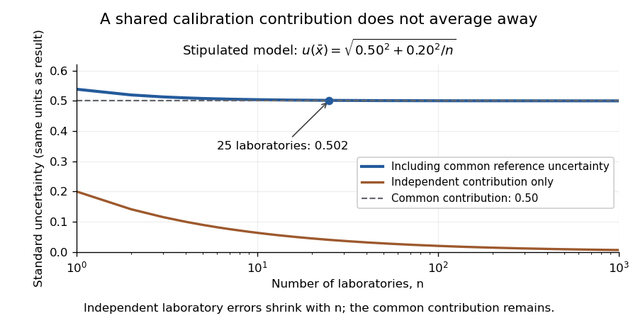
An original interlaboratory uncertainty model: a common calibration contribution remains as independent laboratory variation averages down
. Details. Completeness of an interactive proof guarantees that true statements can convince the verifier in an interactive proof when the designated prover in an interactive proof follows the protocol. For an interactive proof system for a set , a bound requiresPerfect completeness means acceptance probability one on every true input. This is different from soundness of an interactive proof, which concerns every cheating strategy on false inputs.[ref]
An original three-run example shows that a repetition rule changes the guarantee. Suppose three independent runs on a true statement each accept with probability . Requiring all three to accept givesAccepting when a majority does givesThe coefficient counts which one of the three runs rejects in an exactly-two-acceptance outcome. These stipulated independent trials illustrate the aggregation rule; the soundness of the majority rule must be assessed separately.
Thus lowering the chance of false acceptance is not the only design objective. A verifier that always rejects has excellent false-statement behavior but no useful completeness. A successful proof system needs both sides of its acceptance guarantee.
Soundness of an interactive proof bounds how often a verifier in an interactive proof can be induced to accept a false statement. For every false input and every cheating prover in an interactive proof strategy , an acceptance bound requiresIn the usual interactive proof system definition, the quantifier includes computationally unrestricted cheating strategies. Bounding only one tested strategy is insufficient.[ref]
An original repetition example shows why conditional bounds matter. Suppose a single fair bit is reused in two tests, and both accept exactly when . Each test separately accepts with probability , but both accept with probability , not . Merely multiplying marginal probabilities would be wrong.
Instead, if every next test has acceptance probability at most conditional on every preceding accepting history, the chain rule for probabilities giveswith the first term unconditional and zero-probability histories handled trivially. For and , the bound is . The relevant protocol must justify those conditional bounds, rather than assuming that repetition automatically makes every transcript independent.
Soundness protects the false-statement side of verification. It neither guarantees acceptance of true statements nor establishes that a successful interaction hides a cryptographic witness; those are separate completeness and zero-knowledge proof questions.
A prover in an interactive proof is the participant that sends messages intended to convince a verifier in an interactive proof of a public statement. Formally it is a strategy: its next response can depend on the public input, the preceding conversation and any private information or randomness it has. The basic interactive proof system model does not impose the verifier's polynomial time bound on this strategy.[ref]
Probabilistic Proof Systems: A Primer by Oded Goldreich. Sections1.1.2–1.2 and1.5, prover strategies and computational resources
An honest prover follows a designated strategy supporting completeness of an interactive proof. A cheating prover may depart from it; soundness of an interactive proof must still hold for every allowed cheating strategy. Calling a participant a prover therefore does not mean that its assertions are trusted.
A cryptographic witness can make an otherwise difficult response easy to produce. For an original composition example, let be a known graph isomorphism. If the prover sends for a chosen permutation , it can supply as an isomorphism from to , or as an isomorphism from to . Neither response requires solving a new isomorphism search problem from scratch.
Thus a theoretical allowance of unlimited prover computation is different from a claim about implementation cost. Some protocols have efficient honest provers when the witness is supplied; others are studied primarily for the verification power they demonstrate.
A verifier in an interactive proof is the efficient participant that evaluates a public statement using messages from a prover in an interactive proof and its own random choices. Its algorithm specifies which challenge to send, how to process the response and when to accept or reject. In the standard model it runs in probabilistic polynomial time in the public input length.[ref]
The verifier's guarantee concerns more than one successful conversation. Completeness of an interactive proof requires a suitable honest prover to succeed on true statements. Soundness of an interactive proof bounds success of every cheating strategy on false statements. A verifier that accepts whenever it receives any message meets neither requirement merely by being fast.
For an original checking example, suppose a response claims a graph isomorphism between two20-vertex graphs encoded by adjacency matrices. Checking that the vertex mapping is a bijection and that all adjacency entries agree with their mapped entries verifies that response. It does not require searching through all vertex permutations.
An interactive proof system can use such inexpensive checks in a randomized conversation. The verifier's random choices must follow the specified protocol: exposing a challenge too early, reusing randomness in an unjustified way or changing the acceptance rule can alter its mathematical guarantees.
The general intelligence factor, conventionally , is a latent variable used to account for shared variation among performances on different cognitive tasks. Charles Spearman's 1904 analysis distinguished a common component from task-specific contributions, helping establish the historical basis of this approach.[ref]
General Intelligence, Objectively Determined and Measured by Charles Spearman. 1904, chapter V, correlation and common versus specific components
A simple one-factor measurement model writes a standardized test score aswhere is a factor loading. Suppose all variables have zero mean, , each has zero covariance with , and distinct residuals have zero covariance with one another. Then for different tests,Thus a single shared component can explain correlated scores even when the tests contain different content. The covariance equation follows from the stated assumptions; it does not identify a unique biological cause of the correlations.
Factor analysis estimates such models and evaluates their fit. The general intelligence factor should also be distinguished from a first component obtained by principal component analysis: one is a proposed latent structure with residual assumptions, while the other is a variance-maximizing summary of observed scores. Interpretation requires the tasks, population and measurement assumptions, rather than a number alone.
The elliptic-curve factorization method searches for a nontrivial divisor of a composite integer by doing elliptic curve arithmetic modulo . Hendrik W. Lenstra's method replaces the multiplicative group in Pollard's p-1 algorithm with a group whose order varies as the curve varies. For an unknown prime divisor , a curve for which the order of the chosen point has only small prime factors can make a suitably chosen multiple of that point vanish modulo without vanishing modulo every prime divisor of .[ref]
In affine-coordinate arithmetic, trying to invert a denominator modulo can fail. Computing the greatest common divisor then yields a factor if . A full gcd of is inconclusive; another curve or point may be needed. Implementations can accumulate this information with projective coordinates rather than attempting an inversion at every step.
For a small worked example, take , the curve , and . Its discriminant is coprime to . The usual addition formulas give and modulo . Adding these to form calls for inversion of . Since , the failed division exposes a prime divisor. This elementary example illustrates the mechanism; the method's practical advantage is its dependence on the size of the factor sought, rather than only on the size of .
An autoxidation inhibition period is a defined interval during which oxidation is suppressed relative to a matched uninhibited reaction. In an inhibited autoxidation assay, it can report how long a radical-trapping antioxidant retains effective capacity, but the operational start and end of the interval must be specified.
For a limiting model with antioxidant concentration , trapping stoichiometry and constant effective chain-initiation rate , let . If trapping is rapid and quantitative until exhaustion,At chosen values , and , the model gives . Equal periods can arise from different combinations of concentration, stoichiometry and initiation rate, so an independent autoxidation initiation-rate calibration is needed to infer a capacity.
For changing initiation rate, capacity is consumed according to the integrated flux:An original decaying-flux example takes , with . Thenwhen . For , and , this gives about , rather than the initial-rate approximation .
Initiator-limited antioxidant exhaustion arises because this model supplies only total flux . Here that limit is : a capacity would never be exhausted by this modeled initiation source. Absence of a breakpoint would not demonstrate unlimited antioxidant capacity.
Experimentally, a delay can be defined by a stated curve-fitting or threshold rule, while the suppressed region can retain a nonzero oxidation slope. Primary spectrophotometric co-autoxidation work treats kinetics and stoichiometry as distinct properties of the radical-trapping reaction.[ref]
A Continuous Visible Light Spectrophotometric Approach To Accurately Determine the Reactivity of Radical-Trapping Antioxidants by Evan A. Haidasz and others. Indexed abstract, continuous reaction monitoring and kinetic/stoichiometric distinction
A longer apparent period can also reflect changed initiation, oxygen depletion or a readout effect. Comparing a matched blank, a reference antioxidant and a concentration series helps test which interpretation is supported.Autoxidation initiation-rate calibration estimates the effective rate at which radical chains enter the specified inhibited autoxidation assay. It connects a measured inhibition delay to chemical trapping capacity. Initiator concentration by itself is not necessarily this effective rate: decomposition, radical escape and reaction conditions can affect how many chains are actually initiated.
For a known reference radical-trapping antioxidant at concentration with trapping stoichiometry , assume constant effective initiation rate and rapid, quantitative trapping until exhaustion. Capacity balance givesThis calibrates the initiation rate only to the extent that the reference stoichiometry and the inhibition-period interpretation are valid. A single unknown antioxidant cannot generally determine both its own trapping capacity and .
Autoxidation lag standard addition can expose a background capacity. Under an additive-capacity model,An original series with added reference concentrations , and and measured periods , and has slope . For , this implies . The intercept represents an equivalent pre-existing trapping capacity under this model; it does not identify the background chemical species.
Using without accounting for the intercept would give about and at the two nonzero additions, instead of the common slope-based value. A concentration series therefore tests more than one isolated lag measurement. Curvature or changing slopes can indicate that addition changes the chemistry or that the initiation rate is not constant.
The signal still needs a reaction model. A primary visible-light method follows a BODIPY-based signal carrier co-autoxidizing with a hydrocarbon substrate, distinguishing radical-trapping kinetics from stoichiometry.[ref]
A Continuous Visible Light Spectrophotometric Approach To Accurately Determine the Reactivity of Radical-Trapping Antioxidants by Evan A. Haidasz and others. Indexed abstract, signal-carrier method and kinetic/stoichiometric distinction
A fitted optical breakpoint is not automatically the instant of chemical exhaustion.For time-dependent initiation, the balance becomes . Temperature, solvent, oxygen availability, reference identity and the observation procedure must therefore remain controlled or explicitly modeled. The calibration belongs to the assay conditions, rather than being an intrinsic constant transferable to every oxidation experiment.
A spikelet is a small unit of the inflorescence of a grass, containing one or more florets on a short axis. Usually a pair of glumes occurs at the base, and each floret is associated with a lemma and palea.[ref]
This hierarchy matters when counting. An apparent “grain-bearing unit” can be a spikelet with several flowers, so counting spikelets is not generally the same as counting flowers or mature seeds. To inspect one, separate the basal glumes and then examine the individual florets inside. The nested organization links a recognizable cereal head to the reproductive structures of other angiosperms.
Conversion bookkeeping for binary copolymers uses conserved component amounts to distinguish initial feed, residual feed and cumulative incorporated composition. It is an accounting constraint on a closed batch, separate from the kinetic prediction supplied by the copolymer composition equation.
Normalize initial total monomer amount to one mole. Let be its type-1 mole fraction, total molar conversion and the type-1 fraction in the remaining pool. Assume no additional feed, side losses or consumption outside the material being counted. The incorporated amounts areTheir sum is , so the cumulative type-1 fraction isThis is a molar-unit balance; conversion by mass requires the corresponding component molar masses. The IUPAC terminology distinguishes instantaneous composition from integrated conversion/composition relationships.[ref]
IUPAC Compendium of Chemical Terminology, fifth edition (Gold Book). Copolymerisation composition equation, entry 15391, integrated forms and composition drift
For an original example, choose , and residual . The incorporated amounts are 0.05 and 0.45 mol, giving . Individual monomer conversions are and . The residual mixture becomes richer in the less-consumed component even though the polymer contains less of it than the initial feed.
Nonnegative incorporated and remaining amounts impose, for ,For and , a reported residual fraction of 0.50 is impossible under the assumptions: it would leave mol of type 1 when only 0.20 mol was present initially.
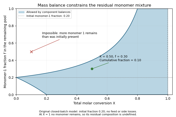
Conserved monomer amounts bound residual-feed composition at each conversion
. Original closed-batch molar bookkeeping for initial type-1 fraction 0.20. The feasible region requires both consumed amounts to be nonnegative; no reaction-rate constants are fitted. Residual composition is undefined at complete conversion. Details.For a differentiable conversion trajectory, the instantaneous fraction is . Equivalently, . This is the bridge between conservation and kinetic composition drift. At complete conversion there is no residual mixture to assign an value; the total incorporated composition nevertheless equals under the closed-batch assumptions. The IUPAC experimental recommendation measures conversion and composition separately rather than replacing both by an initial feed label.[ref]
Radical Copolymerization Reactivity Ratios by IUPAC. Official recommendation announcement, conversion and composition observations
mRNA display is an in vitro selection method in which a peptide or protein is covalently linked to the messenger RNA encoding it. Selecting the displayed molecule can therefore retain recoverable sequence information about that same molecule: a physical genotype-phenotype linkage.
In the original experiment, synthetic messenger RNA carried puromycin at its 3′ end. During translation, this peptide acceptor enabled fusion of the message to its encoded peptide. Richard W. Roberts and Jack W. Szostak tested the linkage by selecting an encoded myc epitope tag with an antibody.[ref]
RNA-peptide fusions for the in vitro selection of peptides and proteins by Richard W. Roberts and Jack W. Szostak. Abstract; Figures 1 and 4, fusion construction and immunoprecipitation
The experimental readout went beyond observing binding. Following immunoprecipitation, reverse transcription and polymerase chain reaction recovered the encoding information. A restriction enzyme distinguished the selected myc sequence from background pool sequences, allowing before-and-after enrichment to be measured.[ref]
RNA-peptide fusions for the in vitro selection of peptides and proteins by Richard W. Roberts and Jack W. Szostak. Selective Enrichment of an RNA-Peptide Fusion and Figure 5
This tests whether selection of a molecular property can recover the associated sequence; it does not establish that every possible sequence displays equally well.An original statistical sampling calculation distinguishes nominal input size from effective displayed-library coverage. Suppose independent input molecules contain a desired sequence class with probability , and each such molecule forms a usable fusion with probability . Before any binding selection,For , and stipulated , the expected usable desired count is only one and the chance of none is approximately 36.8%. Raising the hypothetical yield to 0.10 raises the expected count to ten and reduces that probability to approximately 0.00454%. These are constructed independent-sampling examples, not fusion yields claimed for the original experiment.
Sequence-dependent translation, fusion formation, recovery and amplification can each change representation. A large input sequence pool is therefore different from a large usable displayed pool. Repeating selection and amplification can enrich retained variants, while an independent functional or binding affinity measurement tests whether the recovered sequence has the intended property.
Pinned article: Introduction to the OurBigBook Project
Welcome to the OurBigBook Project! Our goal is to create the perfect publishing platform for STEM subjects, and get university-level students to write the best free STEM tutorials ever.
Everyone is welcome to create an account and play with the site: ourbigbook.com/go/register. We belive that students themselves can write amazing tutorials, but teachers are welcome too. You can write about anything you want, it doesn't have to be STEM or even educational. Silly test content is very welcome and you won't be penalized in any way. Just keep it legal!
Intro to OurBigBook
. Source. We have two killer features:
- topics: topics group articles by different users with the same title, e.g. here is the topic for the "Fundamental Theorem of Calculus" ourbigbook.com/go/topic/fundamental-theorem-of-calculusArticles of different users are sorted by upvote within each article page. This feature is a bit like:
- a Wikipedia where each user can have their own version of each article
- a Q&A website like Stack Overflow, where multiple people can give their views on a given topic, and the best ones are sorted by upvote. Except you don't need to wait for someone to ask first, and any topic goes, no matter how narrow or broad
This feature makes it possible for readers to find better explanations of any topic created by other writers. And it allows writers to create an explanation in a place that readers might actually find it.
Figure 1. Screenshot of the "Derivative" topic page. View it live at: ourbigbook.com/go/topic/derivativeVideo 2. OurBigBook Web topics demo. Source. - local editing: you can store all your personal knowledge base content locally in a plaintext markup format that can be edited locally and published either:This way you can be sure that even if OurBigBook.com were to go down one day (which we have no plans to do as it is quite cheap to host!), your content will still be perfectly readable as a static site.
- to OurBigBook.com to get awesome multi-user features like topics and likes
- as HTML files to a static website, which you can host yourself for free on many external providers like GitHub Pages, and remain in full control

Figure 2. You can publish local OurBigBook lightweight markup files to either OurBigBook.com or as a static website.
Figure 3. Visual Studio Code extension installation.
Figure 5. . You can also edit articles on the Web editor without installing anything locally. Video 3. Edit locally and publish demo. Source. This shows editing OurBigBook Markup and publishing it using the Visual Studio Code extension. 
- Infinitely deep tables of contents:




All our software is open source and hosted at: github.com/ourbigbook/ourbigbook
Further documentation can be found at: docs.ourbigbook.com
Feel free to reach our to us for any help or suggestions: docs.ourbigbook.com/#contact