Topics (384k) Articles (398k) Users (410) Discussions (242) Comments (383) Files (13k) New article

Use local east, north, and up unit vectors , with . In a spherical-Earth approximation at geographical latitude , the angular velocity has components . Expanding the cross product for relative velocity givesThese are Coriolis acceleration components, not the total acceleration. For horizontal motion, the horizontal part is , where the Coriolis parameter is . Thus northward motion in the northern hemisphere has an eastward Coriolis acceleration, to the right of its velocity; in the southern hemisphere the horizontal turning is to the left. At the equator , but the full Coriolis acceleration need not vanish: vertical or eastward motion still couples through .
For a numerical example, take the Earth rotation rate , geographical latitude , and an initially northward relative velocity . Then
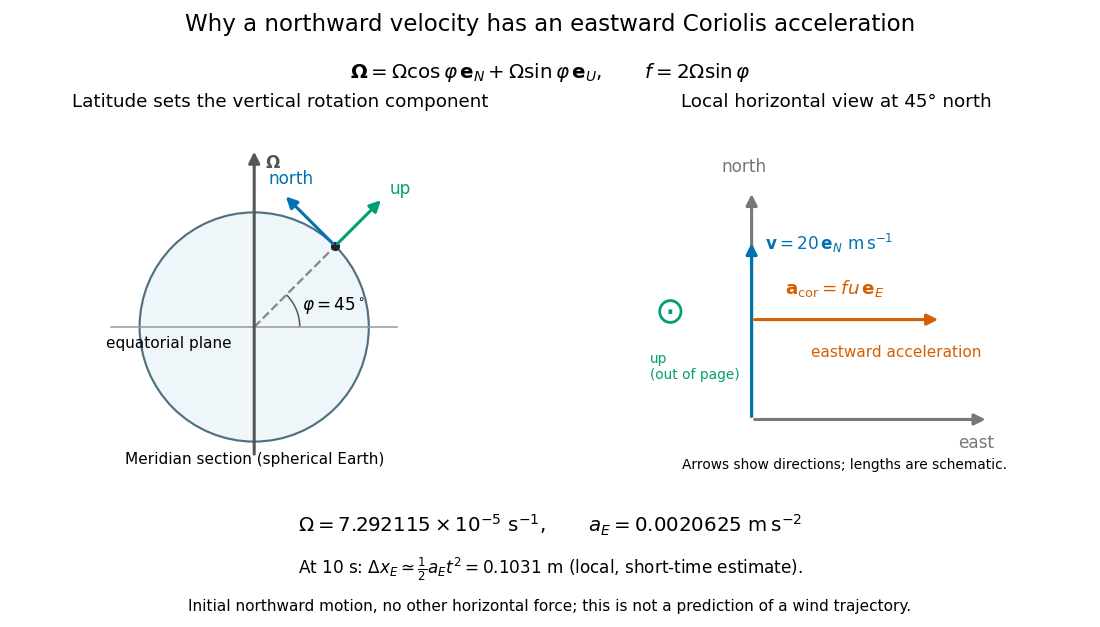
Latitude, local rotation geometry, and the scale of eastward Coriolis acceleration for northward motion
. Details. For a local, short-time estimate with no other horizontal force and zero initial eastward velocity, hold the initial northward velocity in the leading term: . At this gives about eastward. It assumes nearly fixed local axes and geographical latitude, negligible changes of height, and . It is not a complete wind trajectory: pressure gradients, friction, and evolving velocity must enter an atmospheric equation of motion. The effective gravity in a rotating frame already combines ordinary gravity with the steady terrestrial centrifugal acceleration.
Consider a ball moving horizontally with no net horizontal force in the laboratory. Treat its horizontal motion as that of a free particle: with constant . Axes rotating counterclockwise at constant angular velocity about the launch point assign it the positionThis is an exact rotation matrix transformation, with the axes coinciding at . Taking , , and gives the two views below. At , the laboratory position is , but the rotating position is approximately . Both assign the same distance from the origin.
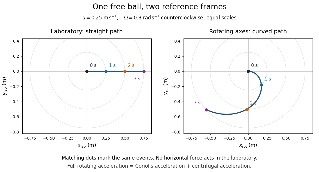
The entire rotating acceleration must include the centrifugal acceleration as well as the Coriolis acceleration. To see the balance explicitly, write and . Direct differentiation givesThe two apparent contributions areAt launch , so only the Coriolis acceleration contributes to the initial bending. Later the centrifugal acceleration also contributes; the full curved trajectory cannot be explained by keeping only the Coriolis force. In particular, grows even though the Coriolis force does no work: the rotating-frame kinetic energy increase is supplied by work from the centrifugal force. The laboratory kinetic energy remains .
SN 1987A supplied a prompt terrestrial record of neutrino emission from a core-collapse supernova through its SN 1987A neutrino burst.[ref]
Nobel Lecture: Birth of neutrino astrophysics by Masatoshi Koshiba. p. 1015: supernova signal and collapse interpretation
A pairing gap is an energy scale for fermionic excitations above a paired superfluid or superconductor ground state. In a simple isotropic paired system the quasiparticle dispersion has the form , where measures the unpaired single-particle energy relative to the chemical potential. A nonzero minimum gap gives exponentially small fermionic thermal occupations when . If the gap varies with direction and has nodes, gapless directions can instead produce power-law thermodynamics. Collective excitations must be counted separately from the gapped fermionic quasiparticles.
For and , split the convolution integral at and . The three contributions are , and . Evenness gives the displayed answer for all real .
With Fourier transform convention , one has . The convolution theorem and Fourier inversion theorem therefore yieldThe value at is . Multiplying by instead gives a normalized Laplace distribution; its self-convolution is the density .
If the partial sums tend to a finite limit , then . Thus failure of the terms to tend to zero proves divergence. The converse is false: the harmonic series has terms tending to zero but diverges.
For two equal point masses joined by a light tether of length , the central moment of inertia is . With conserved angular momentum , the rotational kinetic energy is . Slow, smooth contraction gives with the displayed leading tension. The exact radial correction is and , so the total work-energy theorem remains exact for non-quasi-static schedules too.
Directly scanning all edges to evaluate each child of each of choices takes elementary operations, in Big O notation. There is a faster implementation. When assigning vertex , let and count its already assigned graph neighbours labelled zero and one. Contributions from edges not incident to are unchanged, and contributions from edges to unassigned graph neighbours stay for either choice. ThereforeChoose zero if , otherwise one: put on the side with fewer already assigned graph neighbours. With adjacency lists, scanning each vertex's list once costs operations overall and uses storage including the graph. These bounds count operations on labels and counters that fit in machine words of bits. Multiplying the conditional expectation cut formula by two also permits exact integer comparisons without rounding.
If is the size of a maximum cut, then . The constructed cut of a graph thus has size at least , an approximation ratio of in the maximization convention. The five-versus-six example illustrates the gap between this guarantee and exact optimization.
For a general randomized algorithm, the averaging proof alone does not establish efficient derandomization. One needs a polynomial number of commitments, an efficient way to find a suitable child at each step, and manageable representations and evaluation costs for the relevant conditional expectations. Those evaluations can themselves be hard. Enumerating all completions verifies this small example, but would take exponentially many assignments as grows. The polynomial-time algorithm here comes from the local conditional expectation cut formula, not from that enumeration.
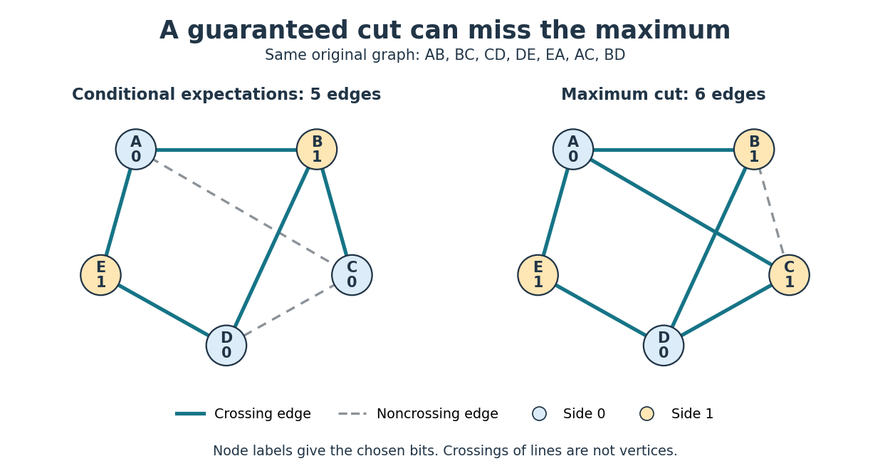
Consider the following original five-vertex simple graph, where denotes the undirected edge :Its seven edges give initial expected value . Use vertex order and choose zero whenever the two child conditional expectations tie.
The complete decision ledger is below. A prefix lists fixed labels in vertex order; all later labels remain hypothetically independent fair bits. Each candidate entry is the conditional expectation of the final cut of a graph, including the contribution of unresolved edges.
| Prefix before choice | Next vertex | Set to 0 | Set to 1 | Chosen label | Retained conditional expectation |
|---|---|---|---|---|---|
| Empty | |||||
For example, after , edge is fixed crossing and the other six edges are unresolved, giving . Setting fixes crossing and noncrossing, leaving four unresolved edges: . Setting instead fixes crossing and noncrossing, giving the same conditional expectation.
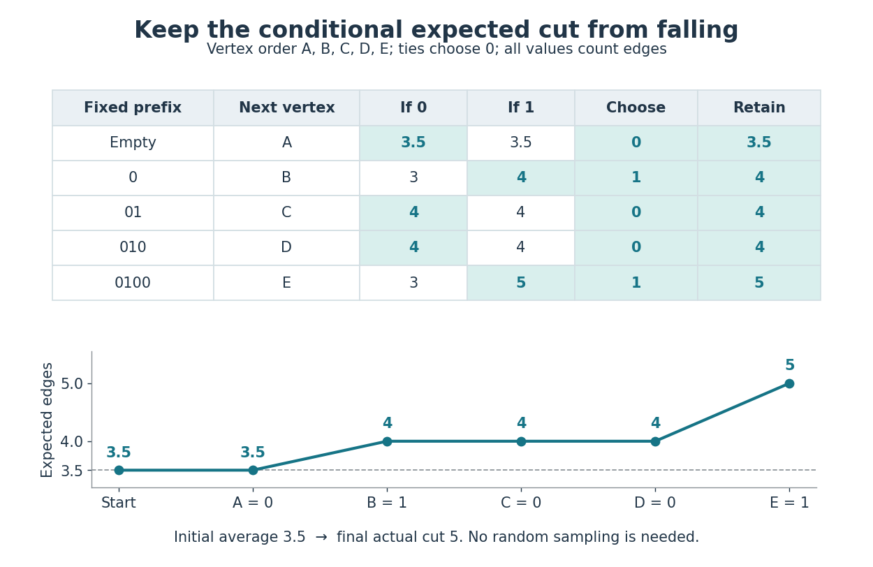
Conditional expected cut values along every chosen branch
. At each step, both candidate values are computed by the conditional expectation cut formula. The highlighted cell is chosen; ties choose zero. Below, the retained conditional expectation follows , starting before any label is fixed. The last value is the actual size of the resulting cut of a graph, rather than an average over remaining choices. Details.The final labels are , so the two sides are and . The five crossing edges are ; do not cross. This exceeds , and hence also the rounded-up guarantee of four edges.
It is not a maximum cut. Labels cross all edges except , giving six. Seven are impossible because the triangle in a graph cannot have all three edges crossing a two-sided cut of a graph. An independent enumeration of all complete label assignments gives the following distribution, counting an assignment and its label-swapped counterpart separately:
| Size of cut of a graph | Number of label assignments |
|---|---|
The weighted sum is , so the average is , agreeing with linearity of expectation. Choosing in the earlier tie discards the remaining size-six completion while preserving the average of four. The method protects an expected value guarantee; it need not preserve the best possible completion.
For any partial assignment , let count edges whose two endpoints are already fixed on opposite sides, and let count edges with at least one unassigned endpoint. Under the remaining independent fair bits,An edge with fixed equal labels contributes zero; fixed unequal labels contribute one. If one endpoint is unassigned, its fair bit disagrees with the fixed label with probability . If both endpoints are unassigned, their independent fair bits disagree with probability as well. Count each unresolved edge once, even when both endpoints are unassigned.
Process vertices in a fixed order. Evaluate the conditional expectation cut formula after setting the next label to zero and after setting it to one; retain the larger value, choosing zero on ties. The conditional expectation choice invariant ensures the final cut of a graph has size at least . This is a deterministic approximation algorithm for maximum cut.[ref]
Lecture notes on randomized approximation algorithms. CS 4820: Algorithms, Spring 2011; Cornell CS 4820, Lecture notes on randomized approximation algorithms, 2 May 2011, §1.1.2, printed pp. 2–3: conditional expectations, Algorithms 1–2 and the half-total-edge-weight guarantee; no individual byline stated
The terms at and are and its negative. Thus the partial sums ending at an odd index are zero, while those ending at equal . Considering both subsequences proves convergence of the full sequence of partial sums, not merely of grouped terms.
The paired sum of absolute values is . Since for , these pairs dominate , whose series diverges by comparison with the harmonic series. The original series therefore has conditional convergence with the displayed sum.
For an ideal chain inside a blob, and . Together with , this gives the displayed concentration-blob size. Under the site-volume approximation , and . The estimate describes local overlap rather than the full chain size and requires for a well-developed semidilute regime.
The imaginary part of the complex refractive index makes wave amplitude decay as . Since intensity is proportional to amplitude squared, its absorption coefficient is .
The real axis consists of the points of the complex plane whose imaginary part is zero. These points represent the real numbers.
A binary operation is noncommutative if some pair of elements fails to commute. Thus reversing their order can change the result. The same operation may still have many commuting elements.
The 2000 experiment prepared optical pulses with a mode-locked laser and broadened them in an air-silica microstructure optical fiber. A wavelength-selective beam splitter separated red and blue light. A nonlinear crystal doubled the red branch; the blue branch received a known acousto-optic shift. A filter selected recombined light for an avalanche photodiode, supplying an electronic beat. Mirror translation controlled repetition frequency; mirror tilt controlled offset with coupled effects. Separate delayed-pulse interference tested programmed phase changes. Alternative envelope fits and unmatched optical reflections were examined as checks and limitations.[ref]
These readouts answer different questions. The electronic beat closes a feedback loop; changing its setpoint and checking the delayed-pulse phase tests whether that control reaches the optical waveform. Neither readout alone establishes the accuracy of an unknown optical frequency. That additionally requires a calibrated time reference, the correct tooth number and beat sign, and checks for missed cycles and drift. The ideal unshifted diagram above omits the experiment's known acousto-optic shift; its actual raw detector frequency must be corrected for that shift before identifying .
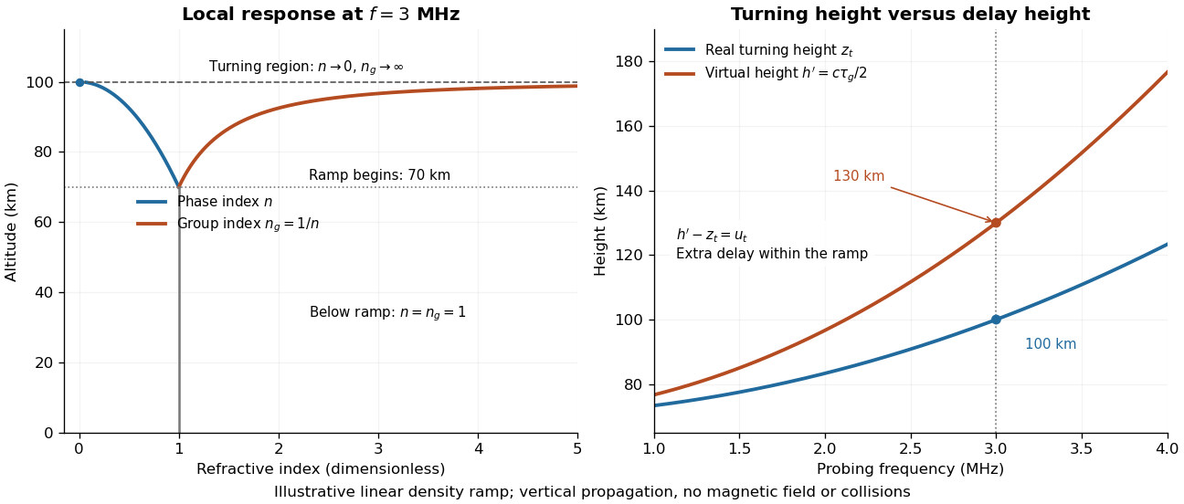
For a vertical outgoing and returning radio wave, define the virtual height from its round-trip group delay , after removing instrument delays. It is the height a fictitious reflector would have if both legs traveled at . It differs from both the real turning height and a height fitted to an oblique constant-path interference fringe model.
An original solvable profile makes the difference explicit. Approximate the region below by , and prescribe a linear rise of squared plasma frequency above it:Here the symbol denotes the penetration depth, and has units . In the propagating part of the ramp, . In the leading geometrical-ray delay model, with a frequency-independent turning connection wave phase, the round-trip group delay isThe endpoint singularity is integrable: substitute to obtain . This approximation does not resolve the finite-wavelength structure at the turning region. It illustrates the effect of slow group velocity before the return, rather than adding extra geometric altitude.
As an independent phase-based derivation, the propagation contribution to the round-trip wave phase isIts derivative agrees with the delay integral. Using the phase integral itself as a distance at speed would give instead of : wave phase, group delay and real turning height are three different quantities.
Choose and stipulate , where . ThenAt , the real turning height is but the virtual height is , corresponding to with . These stipulated parameters describe neither a measured profile nor a separate physical reflector at . Because the ramp has no density maximum, it also has no finite upper penetration threshold; a real bounded E layer or F layer requires a richer profile.
A long coaxial cylindrical capacitor of length and radii has a dielectric-filled overlap of length and relative permittivity . Neglecting end and interface fringing, its filled and vacuum portions are in parallel because both share the same two conductors. The electric potential difference produces in either portion; the electric displacement field and electrode charge differ by the local permittivity. Adding their capacitances gives the title formula. The dielectric boundary is axial while the interior electric field is radial and tangential to that interface, consistent with the electrostatic interface boundary conditions.
In 1961, Raymond Rappaport gently removed membrane and jelly from sand dollar ova with a constricted pipette. After fertilization, he used an inverted optical microscope and rack-and-pinion manipulator to press a needle-mounted glass sphere through an egg onto the chamber floor, producing a torus-shaped biological cell. Visible spindle apparatus positions and cleavage furrow progression were the readout.[ref]
Experiments concerning the cleavage stimulus in sand dollar eggs by Raymond Rappaport. Experiments concerning the cleavage stimulus in sand dollar eggs, pp. 81–82, Materials and Methods: egg preparation, inverted microscope and sphere manipulation
First cytokinesis opened one side into a horseshoe containing two cell nuclei. During the next division, daughters separated from its free ends; an additional cleavage furrow crossed between mitotic asters of different spindle apparatuses. Control eggs supplied the timing comparison. This region lacked intervening chromosomes or a previous nearby spindle apparatus. This supported mitotic aster-associated positioning, without identifying the signal or establishing universal necessity.[ref]
Experiments concerning the cleavage stimulus in sand dollar eggs by Raymond Rappaport. pp. 81–82, introductory experiment summary, Results §1 and Figure 1 legend: horseshoe, second division, control comparison and furrowing between separate mitotic figures
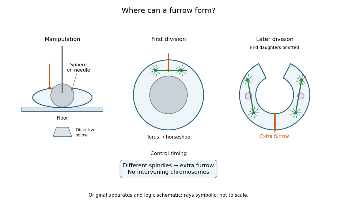
Manipulation and inference in the toroidal sand dollar egg experiment
. Original apparatus and logic schematic; mitotic aster rays are symbolic. Details.For a structureless particle with Hamiltonian , , the classical phase space integral gives the displayed one-particle partition function. Its spatial integral is , while the momentum integral gives . For indistinguishable dilute particles, , , and . These thermodynamic formulas use leading Stirling accuracy; the classical phase-space integral additionally requires temperatures above the discrete trap level scale.
Pinned article: Introduction to the OurBigBook Project
Welcome to the OurBigBook Project! Our goal is to create the perfect publishing platform for STEM subjects, and get university-level students to write the best free STEM tutorials ever.
Everyone is welcome to create an account and play with the site: ourbigbook.com/go/register. We belive that students themselves can write amazing tutorials, but teachers are welcome too. You can write about anything you want, it doesn't have to be STEM or even educational. Silly test content is very welcome and you won't be penalized in any way. Just keep it legal!
Intro to OurBigBook
. Source. We have two killer features:
- topics: topics group articles by different users with the same title, e.g. here is the topic for the "Fundamental Theorem of Calculus" ourbigbook.com/go/topic/fundamental-theorem-of-calculusArticles of different users are sorted by upvote within each article page. This feature is a bit like:
- a Wikipedia where each user can have their own version of each article
- a Q&A website like Stack Overflow, where multiple people can give their views on a given topic, and the best ones are sorted by upvote. Except you don't need to wait for someone to ask first, and any topic goes, no matter how narrow or broad
This feature makes it possible for readers to find better explanations of any topic created by other writers. And it allows writers to create an explanation in a place that readers might actually find it.
Figure 1. Screenshot of the "Derivative" topic page. View it live at: ourbigbook.com/go/topic/derivativeVideo 2. OurBigBook Web topics demo. Source. - local editing: you can store all your personal knowledge base content locally in a plaintext markup format that can be edited locally and published either:This way you can be sure that even if OurBigBook.com were to go down one day (which we have no plans to do as it is quite cheap to host!), your content will still be perfectly readable as a static site.
- to OurBigBook.com to get awesome multi-user features like topics and likes
- as HTML files to a static website, which you can host yourself for free on many external providers like GitHub Pages, and remain in full control

Figure 2. You can publish local OurBigBook lightweight markup files to either OurBigBook.com or as a static website.
Figure 3. Visual Studio Code extension installation.
Figure 5. . You can also edit articles on the Web editor without installing anything locally. Video 3. Edit locally and publish demo. Source. This shows editing OurBigBook Markup and publishing it using the Visual Studio Code extension. 
- Infinitely deep tables of contents:




All our software is open source and hosted at: github.com/ourbigbook/ourbigbook
Further documentation can be found at: docs.ourbigbook.com
Feel free to reach our to us for any help or suggestions: docs.ourbigbook.com/#contact