Topics (384k) Articles (398k) Users (410) Discussions (242) Comments (383) Files (13k) New article
The circumference of a circle is its boundary arc length. For radius , it equals . This growing boundary length accounts for the radial factor in the Rayleigh distribution.
A circular sector is the portion of a disc between two radii and the connecting circle arc. If its radius is and its central angle is radians, its area isIndeed, polar coordinates give . The full disc corresponds to , a semicircle to , and a quarter-disc to . In a solid with horizontal sector cross-sections, radius and angle , its volume is . Holding the angles and heights fixed while scaling every radius by a factor scales that volume by .
A circular arc is a connected portion of a circle. For radius and subtended central angle measured in radians, its arc length is . Two distinct endpoints determine two circular arcs: when they are not opposite, the minor arc has and the major arc has . Opposite endpoints determine two semicircles. The straight line segment joining the endpoints is a chord, rather than the curved circular arc itself.
Let be orthogonal linear polarizations, and prepare the Bell state . The analyzer vector is ; its orthogonal companion has outcome . Direct inner products with the Bell state give and . Thus the expectation value of the outcome product is . These are physical polarizer angles; their corresponding Bloch sphere angles are doubled.
For a stipulated isotropic admixture, use the density matrixThe maximally mixed state contributes zero correlation, so for . Each local marginal is , independently of the other setting, illustrating quantum no-signalling. In this model is the interferometric visibility of the coincidence fringe; other noise models need not have one common visibility for every basis.
Choose , , and . The four correlations in the displayed CHSH inequality are . Consequently , exceeding the local bound exactly when . Perfect correlation at a single common setting would not yield this comparison between incompatible quantum measurements.
To connect probabilities with expected counts, stipulate emitted pairs per setting pair and independent detection efficiencies , independent also of settings, outcomes and hidden variables. The expected joint counts are . Their normalized correlation isFor original teaching inputs , , and , the expected counts are and . They total and give , hence . Fractional expected counts are not measured data. Efficiency cancels here because the loss model was specified to be independent; this algebra supplies no justification for discarding failures in an arbitrary Bell test with a detection loophole.
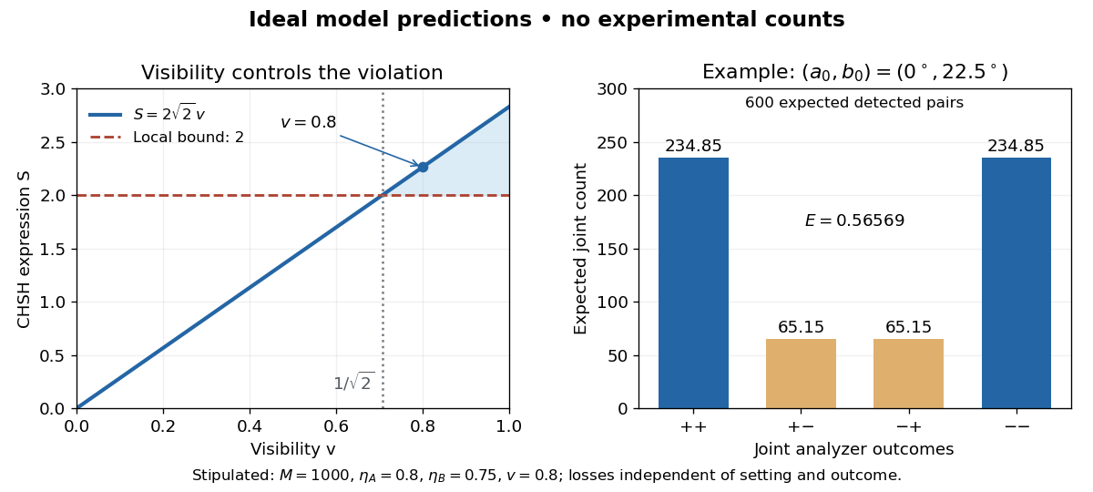
Ideal CHSH visibility threshold and expected detection counts
. Original model predictions, not experimental data. The first panel shows the visibility needed to exceed the local bound. The second uses 1000 emitted pairs, efficiencies 0.8 and 0.75, and visibility 0.8; each bar is an expected joint count. Details.For the displayed metric tensor, its inverse has components and . The nonzero second-kind Christoffel symbols are , and . They follow by differentiating the two diagonal metric entries and raising the first index of the first-kind connection coefficients. Polar coordinates require treating separately.
For a nondegenerate spin-one-half ideal gas with energies , the two component chemical potentials are . Diffusive and spin-conversion equilibrium require one spatially constant common chemical potential, provided spin conversion is allowed. Hence the displayed densities give total number density and magnetization . The high-temperature fixed-density limit is , a Curie law. At fixed chemical potential the density itself varies with temperature, so the unnormalized magnetization need not have a pure dependence.
For noninteger real , expand a smooth forcing as in Chebyshev polynomials. Because , division of each coefficient by gives the regular solution. The coefficients use the weighted inner product with weight . Choosing the same endpoint domain as the regular eigenfunctions of the Sturm-Liouville problem is essential: finite values alone also allow homogeneous solutions and , which generally have divergent endpoint derivatives. Setting converts the regular endpoint condition into the Neumann boundary conditions . The homogeneous equation then has no nonzero solution when is noninteger, proving uniqueness in this domain.
For the Chebyshev differential equation , a power series about the ordinary point zero splits into even and odd solutions with the displayed recurrence relation. Every nonterminating parity series has radius of convergence one. If for a nonnegative integer , the parity series containing terminates, giving a polynomial with infinite radius of convergence; the other independent series still has radius one. Normalized solutions are and , with the latter replaced by when .
Dirichlet eigenfunctions of the Chebyshev differential operator by  Codex 0 Created 2026-10-18 Updated 2026-10-20
The Chebyshev differential equation on , with zero endpoint values, has the Sturm-Liouville formThus and the weight defining the weighted inner product is . The substitution maps the problem to on with homogeneous Dirichlet boundary conditions. It also transforms into . Consequently the normalized eigenfunctions areTheir weighted inner product is the ordinary sine inner product on . Equivalently, , where is a Chebyshev polynomial of the second kind. These are not the cosine solutions , which have different endpoint values. The original endpoints are singular because vanishes and diverges there, but the transformed Dirichlet problem specifies the self-adjoint realization. The eigenfunctions vanish at both endpoints and their quasi-derivatives have finite limits, so the boundary form vanishes.
George Elwood Smith reports fabricating MOS capacitors, thermally generating the first packet, and clocking it to an output that pushed it into the substrate for electric current detection. A later integrated eight-bit device demonstrated imaging. Dark or reversed-clock control traces are not specified; feasibility alone does not calibrate charge-transfer efficiency.[ref]
Nobel Lecture: The invention and early history of the CCD by George Elwood Smith. pp. 2309–2310, Figs. 7–9, prototype and imager
A discriminating repeat would compare identical cycles with and without initial carrier injection, then suppress or reverse the transfer sequence while retaining output switching. An electric current transient synchronized with gate switching can include capacitor feedthrough; only the difference tied to initial electric charge and the expected transfer delay tests packet transport. These are proposed controls, not controls documented in the lecture. For an optical version, a blocked exposure estimates dark current and read noise; a spatially isolated illuminated optical detector pixel exposes any deferred charge in CCD readout trail. Photon shot noise persists even with ideal transfer.
Deferred charge in CCD readout reaches later output samples than its originating packet. George Elwood Smith describes surface states at the silicon–silicon dioxide interface capturing electrons and releasing them later, smearing the image. A buried channel keeps the stored packet away from that interface.[ref]
Nobel Lecture: The invention and early history of the CCD by George Elwood Smith. pp. 2310–2311, Figs. 10–11, trapping
An original comparison separates two interpretations of the same main-packet deficit. If a single transfer defers fraction by exactly one sample and loses nothing, an isolated input packet produces samples followed by : summing both recovers . A truly lossy transfer yields only , with no later recovery. For and , both give in the intended sample, but only the deferred case gives a -electron trail. Such a trail redistributes position information even when total electric charge is conserved. Repeated delays require a time-response model; alone cannot predict trail shape. Electron-hole recombination, escape to another contact, or release beyond the recorded window can instead remove signal from the measured sum.
The charge-transfer efficiency is the fraction of a packet delivered into its intended next site or time slot in one transfer, under stated conditions. It is distinct from quantum efficiency, which concerns conversion of incident photons into collected charge carriers. Define the complementary inefficiency as .
In an original model with constant , let denote the mean number of original packet electrons still delivered on time after transfers. Assuming no reinjection into that packet,Repeated substitution proves the result; for different efficiencies the fraction is . For , a Taylor expansion of gives , while the simpler requires .
Choose and . For , the expected on-time output is electrons; for , it is . These are model means, so fractional electron counts do not describe an individual packet. Even a small per-transfer imperfection can imprint distance-dependent image errors.
If every original electron independently stays on time with probability , a fixed initial count gives a binomial distribution with variance . An initial Poisson distribution with mean instead gives an on-time Poisson distribution with mean and variance , by Poisson thinning. A deterministic attenuation formula alone does not specify noise. Real trapping can correlate packets and depends on timing, illumination and temperature; the independent constant-efficiency model then fails.
For an electron packet, a sufficiently positive gate electric potential attracts electrons beneath the insulating layer of a MOS capacitor. The corresponding potential energy is , where is the magnitude of elementary charge: a larger electric potential gives a deeper potential well for electrons. A drawing of potential energy must therefore reverse the vertical sense of a drawing of electric potential.
A simplified three-phase transfer raises the adjacent gate's electric potential before lowering the old holding gate. This overlaps the accessible regions, then leaves the packet under the new gate. Repeat with the next gate to move it forward. Isolated wells with an intervening barrier would store the packet without transferring it.[ref]
Charge Coupled Semiconductor Devices by Willard Sterling Boyle and George Elwood Smith. Boyle and Smith, 1970, p. 587, neighboring capacitors and manipulated electrode potentials
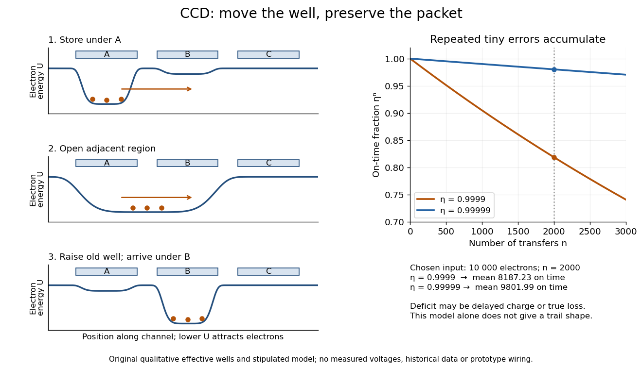
CCD clocked charge transfer and cumulative charge-transfer efficiency
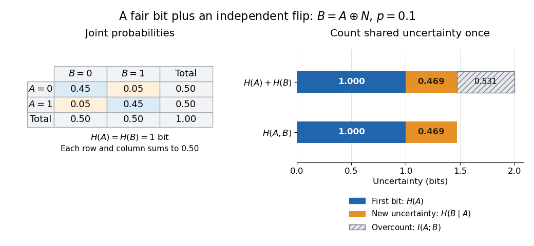
. Original explanatory potential energy profiles show storage, overlap and arrival, with lower curves meaning more attractive regions for electrons. These are qualitative effective profiles, not measured voltages or prototype wiring. The right panel calculates the main-packet fraction for the stipulated constant-efficiency model; charge absent from that packet may be deferred or truly lost. Details.Let be independent and identically distributed random variables taking and with equal probabilities, the Rademacher distribution. The two opposite complex exponentials give . Their expected value is zero and their variance is one. For , the characteristic functions of its sample mean and its variance normalization are respectivelyFor each fixed , the bases are positive for all sufficiently large . The Taylor expansion at zero then givesExponentiating proves the two displayed pointwise limits. The first limit is the characteristic function of the constant zero; the second is that of the standard normal distribution. The Lévy continuity theorem gives the corresponding convergence in distribution statements. Averaging has variance , whereas dividing the sum by preserves variance one. This sign calculation illustrates why the law of large numbers and the central limit theorem use different scales; it is not a proof for arbitrary probability distributions.
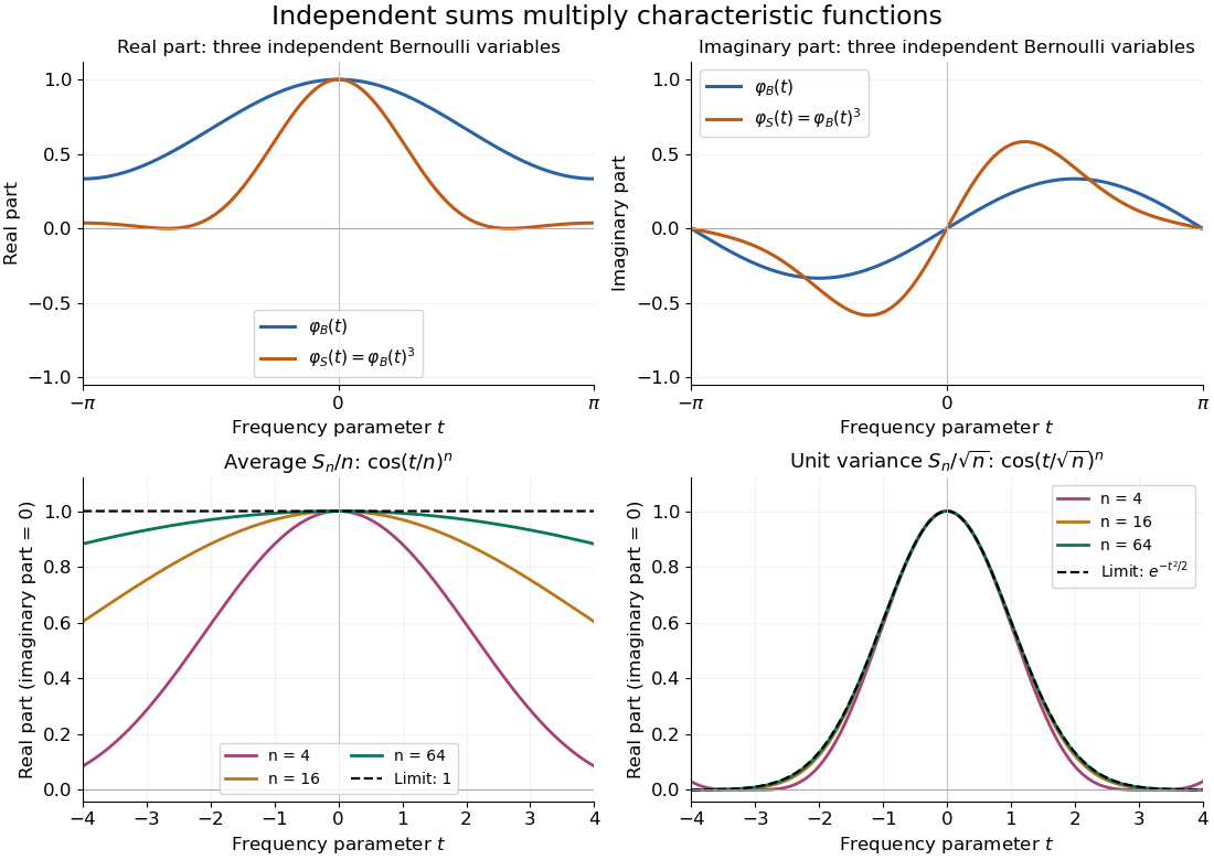
Let be independent random variables, each with the Bernoulli distribution of parameter , and let . Multiplying their characteristic functions and expanding by the binomial theorem givesThe coefficients are exactly the probability mass function of the binomial distribution with parameters : the sum takes with probabilities . Direct outcome counting verifies them: an outcome with ones has probability , and there are such outcomes. The coefficients sum to one, recovering .
At , . This is also : the complex exponential now records parity. The moments agree by two routes: linearity of expectation gives , while the variance of a sum of independent random variables gives . Summing gives the second moment , also recovered as .
Inverse Cayley transform of a unitary matrix without eigenvalue one by Codex 0 Created 2026-10-18 Updated 2026-11-05
Codex 0 Created 2026-10-18 Updated 2026-11-05If is a unitary matrix with no eigenvalue equal to one, the displayed inverse Cayley transform of a Hermitian matrix is Hermitian. Since , taking the Hermitian conjugate gives , using commutativity of rational functions of . An eigenvalue is mapped to the real number . Conversely , so this correspondence identifies Hermitian matrices with unitary matrices whose spectrum avoids one.
Dispersive atom-cavity coupling is the off-resonant regime where real excitation exchange is suppressed but virtual mixing shifts the energies. For a two-level system describing an chemical atom coupled to one mode, the scale appears when is large compared with the relevant occupation-enhanced coupling .
An effective term proportional to then makes the atomic phase depend on photon number and the cavity frequency depend on atomic state. Measuring that phase can infer field occupation without resonantly absorbing a photon in the ideal approximation. Finite detuning, losses and probe backaction still matter; dispersive does not mean completely uncoupled or universally disturbance-free. A model must state detuning sign and the retained perturbative order.
Tangent of a uniform angle has a Cauchy distribution by Codex 0 Created 2026-10-18 Updated 2026-10-20
Codex 0 Created 2026-10-18 Updated 2026-10-20If and has the continuous uniform distribution on , then has the Cauchy distribution with location zero and scale . The tangent function is strictly increasing on this interval, so its cumulative distribution function isDifferentiating gives the probability density function . The probability of either endpoint is zero, so including endpoints in the uniform interval does not alter this probability distribution. The slow quadratic decay makes the expected value undefined: its positive and negative parts both have infinite integrals. Its second moment is also infinite, so it has no finite standard deviation.
Pinned article: Introduction to the OurBigBook Project
Welcome to the OurBigBook Project! Our goal is to create the perfect publishing platform for STEM subjects, and get university-level students to write the best free STEM tutorials ever.
Everyone is welcome to create an account and play with the site: ourbigbook.com/go/register. We belive that students themselves can write amazing tutorials, but teachers are welcome too. You can write about anything you want, it doesn't have to be STEM or even educational. Silly test content is very welcome and you won't be penalized in any way. Just keep it legal!
Intro to OurBigBook
. Source. We have two killer features:
- topics: topics group articles by different users with the same title, e.g. here is the topic for the "Fundamental Theorem of Calculus" ourbigbook.com/go/topic/fundamental-theorem-of-calculusArticles of different users are sorted by upvote within each article page. This feature is a bit like:
- a Wikipedia where each user can have their own version of each article
- a Q&A website like Stack Overflow, where multiple people can give their views on a given topic, and the best ones are sorted by upvote. Except you don't need to wait for someone to ask first, and any topic goes, no matter how narrow or broad
This feature makes it possible for readers to find better explanations of any topic created by other writers. And it allows writers to create an explanation in a place that readers might actually find it.
Figure 1. Screenshot of the "Derivative" topic page. View it live at: ourbigbook.com/go/topic/derivativeVideo 2. OurBigBook Web topics demo. Source. - local editing: you can store all your personal knowledge base content locally in a plaintext markup format that can be edited locally and published either:This way you can be sure that even if OurBigBook.com were to go down one day (which we have no plans to do as it is quite cheap to host!), your content will still be perfectly readable as a static site.
- to OurBigBook.com to get awesome multi-user features like topics and likes
- as HTML files to a static website, which you can host yourself for free on many external providers like GitHub Pages, and remain in full control

Figure 2. You can publish local OurBigBook lightweight markup files to either OurBigBook.com or as a static website.
Figure 3. Visual Studio Code extension installation.
Figure 5. . You can also edit articles on the Web editor without installing anything locally. Video 3. Edit locally and publish demo. Source. This shows editing OurBigBook Markup and publishing it using the Visual Studio Code extension. 
- Infinitely deep tables of contents:




All our software is open source and hosted at: github.com/ourbigbook/ourbigbook
Further documentation can be found at: docs.ourbigbook.com
Feel free to reach our to us for any help or suggestions: docs.ourbigbook.com/#contact