Topics (384k) Articles (398k) Users (410) Discussions (242) Comments (383) Files (13k) New article
For speed in , Fermat principle gives the elapsed-time integrand . Its symmetric stationary light rays through are the displayed catenaries. Set . The endpoint equation is . This function decreases and then increases, with unique minimum where . Thus above the minimum there are two stationary rays, at the minimum one, and below it none. The travel time on either ray is , and its minimum height is .
For and , one solution is , with . A second has , with . Hence these endpoints do not uniquely specify the ray. Stationarity is distinct from global minimization: paths descending almost to have limiting travel time , below either stationary value in this example.
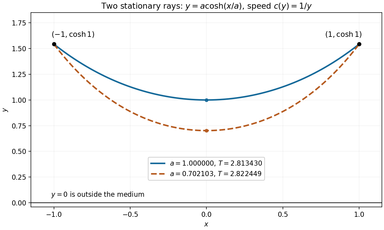
Two stationary catenary rays connect the same endpoints
. For speed , the endpoints and admit stationary light rays with minimum heights and . Their different travel times illustrate that Fermat principle is a stationarity condition. Details.Given injections and , start with the set difference : these are exactly the inputs for which is unavailable. Follow both functions repeatedly, using the natural-number recursion theorem to defineThus contains all the members reachable from any starting point in . The notation and denotes images of a function. If is the empty set, then every is empty and alone gives the desired bijection.
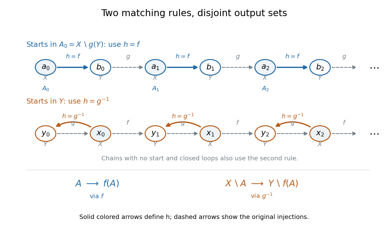
The Injection-chain proof of the Cantor-Schröder-Bernstein theorem partitions the inputs into two matching rules
. The upper row shows a chain seeded in , where the bijection follows . The lower row shows a chain beginning in , where the bijection reverses . The same rule also handles chains with no starting point and closed loops. Separate and copies are used even if the original sets overlap. Details.Define a function on all of byHere is the inverse function from to , obtained by restricting the codomain of to its image. It is well defined because is injective. Every belongs to , since , so the second rule is always available where it is used.
The decisive set identity isThe last equality holds because every with lies in , whereas is disjoint from . Consequently, for any ,Indeed, cannot belong to ; if it lies in , the identity gives for some , and injectivity gives . The converse follows directly by applying .
Now restricts to a bijection from onto . The displayed equivalence says that restricts to a bijection from onto , so its inverse function bijects the remaining inputs with the remaining outputs. The two input sets partition and the two output sets partition . Their combined function is therefore both injective and surjective.
No choice function is needed: is fixed by the given injections, and each required is unique. We neither choose a representative from each chain nor enumerate . This is a proof in ordinary classical ZF, even when no well-ordering of the sets exists there.[ref]
Cantor-Schroeder-Bernstein Theorem by Paul Garrett. Paul Garrett, Cantor-Schroeder-Bernstein Theorem, pp. 1–2, chain construction and pairings; p. 1, no invocation of the axiom of choice
Take , the nonnegative integers, and , the positive integers. Choose the injectionsHere is an inclusion map, while reaches only the positive even integers. In particular, is not a bijection: it misses every positive odd integer. Simply using the inverse function of on its image misses input zero.
The remedy is to follow the alternating injections starting at the missing input zero:The subscripts distinguish an input in from an output in , even when their numerical values agree. The resulting subset of is . Its sequence of members satisfies and , giving by mathematical induction. Define the function
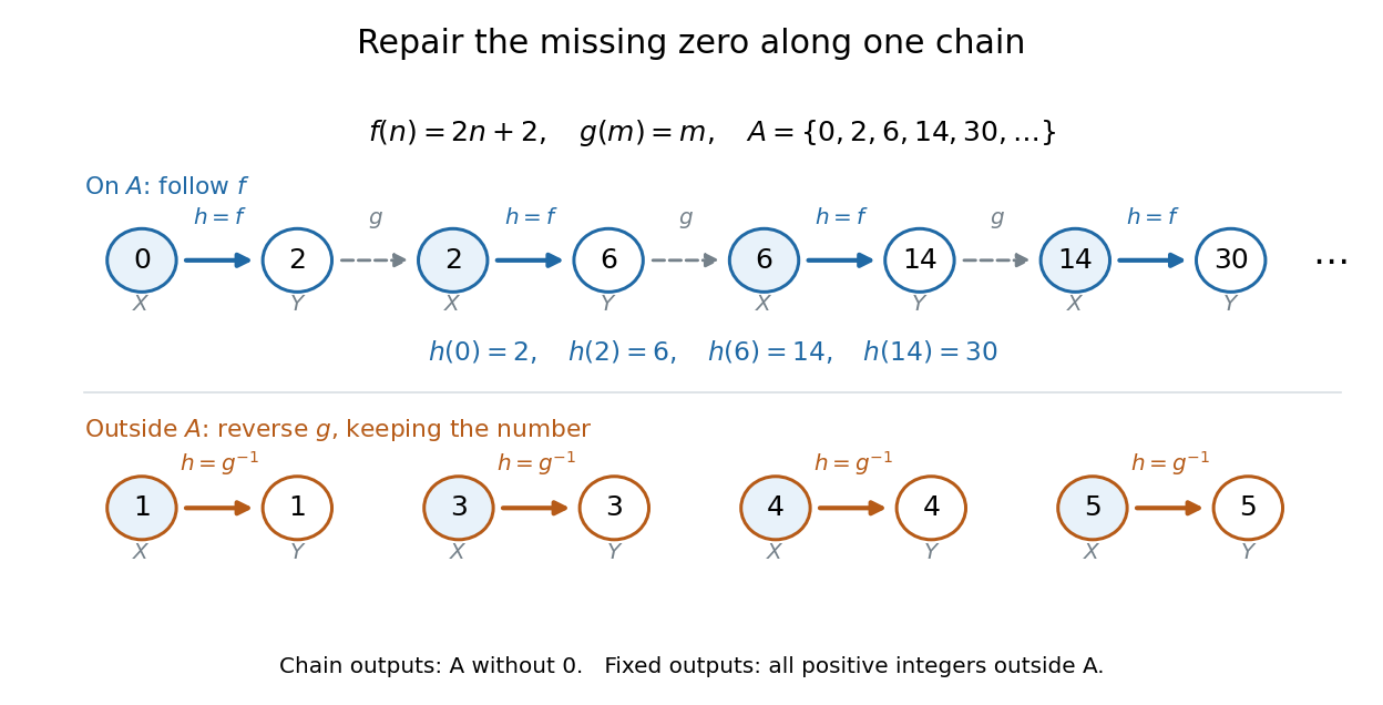
The image covers all the positive members of exactly once. The other inputs cover exactly once by staying fixed. These output sets are disjoint and their union is , proving that is a bijection. In particular, , , , while and .
For completeness, its inverse function isThe familiar bijection also works, but this example shows something more specific: the two chosen injections can repair the missing zero by moving only a sparse sequence of inputs. The repair never has to shift the entire set.
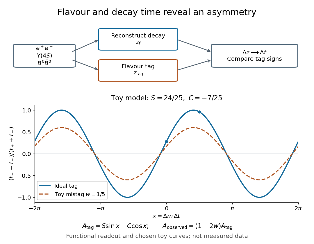
BABAR used asymmetric electron-Positron collisions near the Upsilon meson resonance to prepare neutral B meson pairs. It reconstructed one decay into charmonium plus a kaon, and used flavour tagging on the other B meson with charged leptons or kaons. Silicon tracking reconstructed decay vertices for the decay-time difference. Self-tagging decays calibrated mistags and time resolution; charged decays provided a control. The tagged time distributions established CP violation, limited by backgrounds, mistags and vertex alignment.[ref]
The Lorentz boost converts vertex separation to at leading order. Unequal beam energies thus make a time difference measurable as a distance.[ref]
For a gas of fixed composition in hydrostatic equilibrium, with upward and downward gravitational acceleration of magnitude , an adiabatic process gives the displaced element density change . Comparing with the ambient change yieldsThe ideal gas law and give the title expression, where is the constant-pressure specific heat capacity. A temperature gradient less negative than the adiabatic lapse rate gives positive ; a steeper decline gives convective instability.
A colloidal grain in a liquid is large enough to see with a microscope, yet small enough for thermal motion to compete with its tendency to settle. In the Perrin sedimentation experiment, the equilibrium number density falls with height: a visible miniature atmosphere. Counting grains at different heights measures an energy scale; tracking their Brownian motion measures a transport rate. Connecting both to the same Avogadro constant makes the experiment a quantitative test of kinetic theory. The Wiener measure describes an idealized path law; these measurements instead test a physical model and its material parameters.
Jean Baptiste Perrin's 1909 memoir traces his sedimentation experiments to May 1908. It reports relative counts , , , at heights , , , , and compares radius estimates from Stokes settling velocity, counted grain mass, and rows of touching grains.[ref]
Mouvement brownien et réalité moléculaire by Jean Baptiste Perrin. 1909 memoir, §§15, 20–22; scan pp. 28, 41–49
The 1926 lecture describes resin precipitated from alcohol into water, washed and fractionated by centrifugation to obtain nearly monodisperse gamboge or mastic grains. Diameter and density were measured separately. A sealed slide-and-cover-glass chamber prevented evaporation; a vertical microscope resolved roughly layers through a roughly depth. Refocusing and photographing compared layer populations after equilibrium; changing temperature reversibly changed the distribution.[ref]
Discontinuous Structure of Matter by Jean Baptiste Perrin. Nobel Lectures, Physics 1922–1941; Discontinuous structure of matter, 11 December 1926, pp. 148–150
In Les Atomes (1913), Jean Baptiste Perrin restricts the eyepiece view to fewer than five or six grains and alternates observations between heights. Focus displacement requires a refractive index correction to recover actual layer separation. Horizontal positions were marked with a camera lucida, usually every , and distances calibrated with a micrometer; the polygon joins sampled positions rather than recording the intervening trajectory.[ref]
https://fr.wikisource.org/wiki/Les_Atomes/III. Les Atomes, chapter III, §§61–64
[ref]https://fr.wikisource.org/wiki/Les_Atomes/IV. Les Atomes, chapter IV, §§70–75
A photon-recoil lag correlation asks how often a photon record occurs at a specified time displacement from an electron record. Let be observed separate-channel rates, the rate of detected genuine pairs before a timing cut, and their normalized timing probability density function. For an original dilute, stationary model with observation time , neglecting end effects and detector dead time, the expected pair density isThis counts all pairs of records, rather than at most one detector trigger per electron. It uses independent unrelated detections for the flat term and an added same-event contribution. A normal distribution for timing spread is a chosen approximation, not a claim about the historical instrument. Intrinsic emission delay, counter response and readout uncertainty can all affect the observed probability density function.
Define the accepted lag interval by : is its full width. Integrating the flat baseline gives the existing accidental coincidence expectation . The additional area is . Moving a window of the same full width away from the peak tests the baseline under the model's stationarity assumption. It does not remove correlated instrumental backgrounds or changing rates automatically.
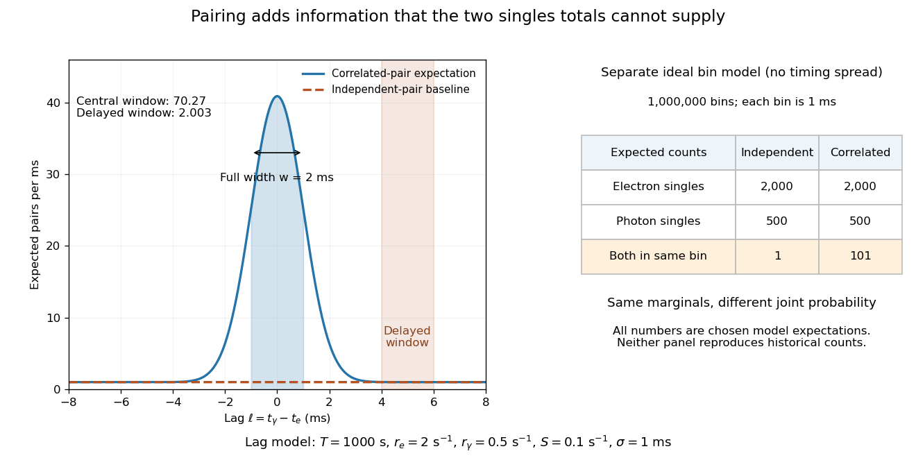
Lag-dependent pairs and a joint probability distribution carry information absent from singles totals
. Original chosen models, not historical counts or fitted data. Left: a normalized normal distribution of genuine-pair lags with standard deviation is added to an independent-pair baseline. Shaded intervals have full width , centered at zero and . Right: a separate exact ideal-bin model ignores timing spread; the two populations have identical singles expectations but different joint expectations. Details.For the lag model, choose , , , and timing standard deviation . A full width gives expected accidental coincidences and accepted genuine pairs, using the error function. The total is approximately , whereas the displaced interval from to has approximately expected pairs. A finite sample fluctuates around these expectations; these values are not measured counts or a significance calculation.
The right panel isolates the information lost by retaining singles totals alone. In a separate idealized model, stipulate independent bins, with Bernoulli distribution indicators for electron and photon detection in a bin. Set and . Independence predicts , hence one expected double detection. Alternatively chooseThese nonnegative probabilities sum to one and preserve both marginal probabilities, yet predict double detections in expectation. Their covariance is . This is an exact joint probability distribution illustrating pairing; it does not model the timing spread in the left panel or reconstruct either historical hypothesis quantitatively. Its lesson is why two singles totals cannot decide whether the observed events share a cause.
In dimensions, isotropic modes with dispersion have density of states proportional to . Their equilibrium number is not conserved, so the excitation chemical potential is zero. Integrating and rescaling by gives the displayed energy power and heat capacity proportional to . In three dimensions, linear acoustic phonons give energy and heat capacity; quadratic gapless ferromagnetic magnons give energy and heat capacity. A gap changes the asymptotically low-temperature law to activated behaviour. The mode approximation applies below the relevant band cutoff and when interactions between excitations are negligible.
The scattering interpretation connects an incoming preparation to the relative frequency of outgoing directions and final atomic states. Max Born's 1926 paper treats a distant incoming electron and a chemical atom, expands the outgoing wavefunction into final atomic states, and imposes conservation of energy. Its translated correction footnote specifies the square of the coefficient; the modern complex modulus notation below is ours.[ref]
Zur Quantenmechanik der Stoßvorgänge by Max Born. Zur Quantenmechanik der Stoßvorgänge, 1926, pp. 863–867; inspected in D. H. Delphenich's translation, pp. 2–4, especially p. 3 equation (1) and footnote 1: squared coefficient
In his 11 December 1954 lecture, Max Born recalled the difficulty of interpreting bound electrons alone. He instead described an incident electron wave generating an outgoing spherical wave, with direction-dependent squared amplitude determining relative scattering probabilities. Distinct final atomic states describe excitation with corresponding electron energy loss. This is a retrospective account of an interpretation, rather than the report of a new apparatus.[ref]
The statistical interpretation of quantum mechanics by Max Born. The statistical interpretation of quantum mechanics, lecture delivered 11 December 1954, printed pp. 261–262; inspected through the transcription at studyres.com/doc/8624145/the-statistical-interpretation-of-quantum-mechanics, paragraphs from the bound-electron difficulty through inelastic scattering
The distinction from the modern Born rule matters. The historical question was which collision outcome occurs: a direction of motion and a final atomic state. The general projective measurement formula applies to arbitrary observables, including degenerate outcomes and mixed states; a positive operator-valued measure describes still more general detector statistics. Those formulations should not be read back as the explicit contents of the short 1926 scattering paper. Nor does the scattering interpretation itself supply a rule for the conditional post-measurement state.
Actual experimental settings are described in the Davisson–Germer experiment and the Franck-Hertz experiment. The former scans collected electric current as an electron beam scatters from prepared nickel; changing direction, accelerating voltage and surface preparation probes electron diffraction. The latter uses acceleration through mercury vapor and a retarding collector to infer discrete energy losses from current minima, with vapor density and retarding settings as controls. Angular resolution and surface backgrounds limit the first inference; initial energy spread and collision positions limit the second. These linked experiments supply the preparation, apparatus and readout; the examples below are original calculations, not Born's measured data.
Bootstrap Methods: Another Look at the Jackknife by Bradley Efron, 1979 journal article appeared in The Annals of Statistics 7(1), pp. 1–26, in January 1979. The original article's bibliographic cover identifies the author, journal, date and pages.[ref]
Bootstrap Methods: Another Look at the Jackknife by Bradley Efron, 1979 journal article. Bibliographic cover: B. Efron, The Annals of Statistics 7(1), January 1979, pp. 1–26
Stanford's earlier technical report BIO 32, also by Bradley Efron and with the same title, is dated July 1977; that report date is distinct from the journal publication date.[ref]Bootstrap Methods: Another Look at the Jackknife by Bradley Efron, BIO 32 technical report. Stanford catalogue: author B. Efron; report BIO 32; report date July 1977
Exact bootstrap distribution for three observations by  Codex 0 Created 2026-10-18 Updated 2026-11-05
Take the original observations , with sample mean . All ordered bootstrap samples have probability . The bootstrap sample has sample mean ; has sample mean ; has sample mean . These are illustrative possibilities, not three simulated measurements used to estimate the distribution.
For bootstrap count vectors , records the number of copies of observed slot . Their multinomial distribution isand . Thus the unordered counts have probability , whereas have probability . Stars and bars gives ten count vectors, but assigning each probability would be wrong. Two different count vectors, and , both give sample mean ; combining their probabilities gives .
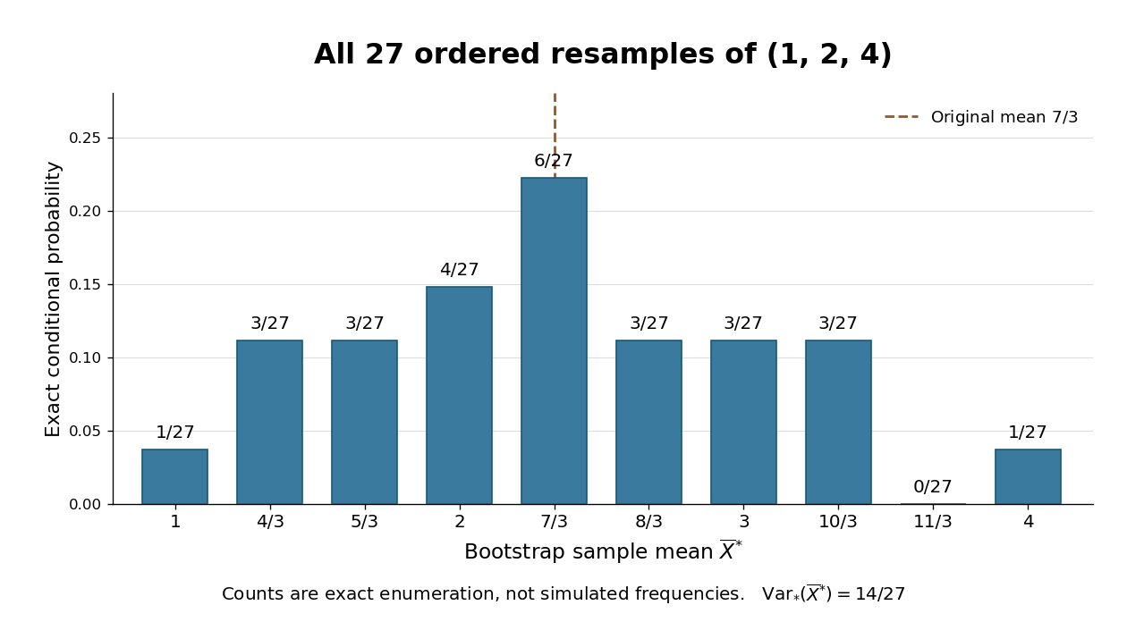
The conditional bootstrap variance of a sample mean gives a compact check on the enumeration. Each resampled draw has expected value and varianceAveraging three independent draws divides that variance by three:The exact conditional bootstrap standard error is . The original sample variance with denominator is , so its usual estimated standard error for the sample mean is . Their squared ratio is here; the difference follows from the empirical measure's denominator , not a numerical simulation error. Neither number is the known true sampling standard error of the unknown source probability distribution.
The part of entropy associated with the number of distinct spatial or occupancy arrangements consistent with chosen macroscopic constraints. For equally weighted configurations, the Boltzmann entropy formula gives the displayed expression. Unequal probabilities require over configurations. For indistinguishable empty sites among otherwise occupied sites, . Vibrational or internal degrees of freedom can contribute additional entropy even at fixed site arrangement.
Blume-Capel mean-field transition at zero single-ion anisotropy by Codex 0 Created 2026-10-18 Updated 2026-11-05
Codex 0 Created 2026-10-18 Updated 2026-11-05For spins with ferromagnetic nearest-neighbour exchange and no single-ion anisotropy, a homogeneous mean-field approximation givesThe self-consistency equation is with . Its small- expansion is . Hence and, with , the nonzero branches satisfy . The critical exponent is the mean-field value , not an exact two-dimensional exponent. At zero source the finite-system equilibrium magnetization is zero by spin inversion symmetry; the broken branches describe the thermodynamic limit with a phase selected by a vanishing source.
For and a nonnegative integer , integration by parts gives, when ,The endpoint term vanishes. ThereforeRepeated application yields . The integration by substitution also identifies with an Euler beta function. A related weighted integral follows immediately from the same substitution:
For positive real , substitute in the defining Euler beta function integral. The increasing substitution maps onto and has . Combining this factor with gives the displayed identity. Positivity of both parameters ensures convergence at the two endpoints, even when the integrand is unbounded there.
In , put . Then , and evenness givesThe further substitution turns this into . The symmetry of the Euler beta function yields the title identity. This proof works for every positive real , without requiring to be an integer or using the Gamma function.
In 2006, Zoran Hadzibabic, Peter Krüger, Marc Cheneau, Baptiste Battelier and Jean Dalibard split a cooled rubidium-87 cloud into two independent planar gases using an optical lattice. After release, the expanding sheets overlapped; absorption imaging recorded their matter-wave interference. Smooth fringe waviness revealed thermal phase fluctuations, while sharp dislocations indicated isolated vortices. The initial evaporative-cooling endpoint controlled the preparation; central fringe contrast served as a degeneracy proxy because direct thermometry in the lattice was difficult.[ref]
Berezinskii-Kosterlitz-Thouless Crossover in a Trapped Atomic Gas by Zoran Hadzibabic and others. Pages 1–2, preparation and readout; Fig. 1; temperature control and Fig. 2
Loss of extended coherence coincided with increased vortex signatures. The optical trap and finite cloud produced a crossover; tightly bound pairs were unresolved, and short-wavelength modes could contaminate high-temperature counts. These were observations of the vortex-unbinding mechanism, not a direct measurement of phase stiffness or a sharp homogeneous universal stiffness jump. The authors left the sample's superfluidity open.[ref]
Berezinskii-Kosterlitz-Thouless Crossover in a Trapped Atomic Gas by Zoran Hadzibabic and others. Pages 3–4, Figs. 3–4; geometry, invisible pairs, detection limits and final paragraph on unmeasured superfluidity
Consider an original counting example: a square two-dimensional XY model of side , a microscopic core radius , and a fixed phase stiffness . This deliberately neglects screening by other vortices. Away from a unit phase vortex, and . Integrating the Goldstone-mode effective free energy over an annulus givesBoundary shape changes finite terms. There are order core positions, so the positional entropy is , where is the Boltzmann constant. With , subtracting gives the displayed free energy.
For and , the dimensionless free energy cost is about at and at . The same logarithm appears in the cost and the positional reward: increasing the system size strengthens whichever has the larger coefficient. The corresponding one-defect Boltzmann factors, about and , are relative statistical weights, not normalized probabilities. The latter signals failure of a dilute single-defect estimate.
A single net phase vortex requires compatible boundaries: on a periodic sample use neutral pairs, as required by vortex charge neutrality. This argument identifies a possible threshold, but predicting the universal stiffness jump requires the renormalized phase stiffness, after smaller pairs have responded. It does not justify setting the transition temperature equal to a bare lattice coupling divided by a universal constant.
The neutral axis is the line in the cross-section of an elastic beam where longitudinal bending strain vanishes. For a homogeneous beam in pure bending, zero resultant longitudinal force gives , so the neutral axis passes through the centroid. Fibres on its opposite sides are stretched and compressed. The second moment of area about this axis controls the relation between bending moment and curvature.
Pinned article: Introduction to the OurBigBook Project
Welcome to the OurBigBook Project! Our goal is to create the perfect publishing platform for STEM subjects, and get university-level students to write the best free STEM tutorials ever.
Everyone is welcome to create an account and play with the site: ourbigbook.com/go/register. We belive that students themselves can write amazing tutorials, but teachers are welcome too. You can write about anything you want, it doesn't have to be STEM or even educational. Silly test content is very welcome and you won't be penalized in any way. Just keep it legal!
Intro to OurBigBook
. Source. We have two killer features:
- topics: topics group articles by different users with the same title, e.g. here is the topic for the "Fundamental Theorem of Calculus" ourbigbook.com/go/topic/fundamental-theorem-of-calculusArticles of different users are sorted by upvote within each article page. This feature is a bit like:
- a Wikipedia where each user can have their own version of each article
- a Q&A website like Stack Overflow, where multiple people can give their views on a given topic, and the best ones are sorted by upvote. Except you don't need to wait for someone to ask first, and any topic goes, no matter how narrow or broad
This feature makes it possible for readers to find better explanations of any topic created by other writers. And it allows writers to create an explanation in a place that readers might actually find it.
Figure 1. Screenshot of the "Derivative" topic page. View it live at: ourbigbook.com/go/topic/derivativeVideo 2. OurBigBook Web topics demo. Source. - local editing: you can store all your personal knowledge base content locally in a plaintext markup format that can be edited locally and published either:This way you can be sure that even if OurBigBook.com were to go down one day (which we have no plans to do as it is quite cheap to host!), your content will still be perfectly readable as a static site.
- to OurBigBook.com to get awesome multi-user features like topics and likes
- as HTML files to a static website, which you can host yourself for free on many external providers like GitHub Pages, and remain in full control

Figure 2. You can publish local OurBigBook lightweight markup files to either OurBigBook.com or as a static website.
Figure 3. Visual Studio Code extension installation.
Figure 5. . You can also edit articles on the Web editor without installing anything locally. Video 3. Edit locally and publish demo. Source. This shows editing OurBigBook Markup and publishing it using the Visual Studio Code extension. 
- Infinitely deep tables of contents:




All our software is open source and hosted at: github.com/ourbigbook/ourbigbook
Further documentation can be found at: docs.ourbigbook.com
Feel free to reach our to us for any help or suggestions: docs.ourbigbook.com/#contact